5 Getting Started with pandas
pandas will be a major tool of interest throughout much of the rest of the book. It contains data structures and data manipulation tools designed to make data cleaning and analysis fast and convenient in Python. pandas is often used in tandem with numerical computing tools like NumPy and SciPy, analytical libraries like statsmodels and scikit-learn, and data visualization libraries like matplotlib. pandas adopts significant parts of NumPy's idiomatic style of array-based computing, especially array-based functions and a preference for data processing without for loops.
While pandas adopts many coding idioms from NumPy, the biggest difference is that pandas is designed for working with tabular or heterogeneous data. NumPy, by contrast, is best suited for working with homogeneously typed numerical array data.
Since becoming an open source project in 2010, pandas has matured into a quite large library that's applicable in a broad set of real-world use cases. The developer community has grown to over 2,500 distinct contributors, who've been helping build the project as they used it to solve their day-to-day data problems. The vibrant pandas developer and user communities have been a key part of its success.
Many people don't know that I haven't been actively involved in day-to-day pandas development since 2013; it has been an entirely community-managed project since then. Be sure to pass on your thanks to the core development and all the contributors for their hard work!
Throughout the rest of the book, I use the following import conventions for NumPy and pandas:
In [1]: import numpy as np

In [2]: import pandas as pd
Thus, whenever you see pd. in code, it’s referring to pandas. You may also find it easier to import Series and DataFrame into the local namespace since they are so frequently used:
In [3]: from pandas import Series, DataFrame5.1 Introduction to pandas Data Structures
To get started with pandas, you will need to get comfortable with its two workhorse data structures: Series and DataFrame. While they are not a universal solution for every problem, they provide a solid foundation for a wide variety of data tasks.
Series
A Series is a one-dimensional array-like object containing a sequence of values (of similar types to NumPy types) of the same type and an associated array of data labels, called its index. The simplest Series is formed from only an array of data:
In [14]: obj = pd.Series([4, 7, -5, 3])

In [15]: obj
Out[15]:
0    4
1    7
2   -5
3    3
dtype: int64
The string representation of a Series displayed interactively shows the index on the left and the values on the right. Since we did not specify an index for the data, a default one consisting of the integers 0 through N - 1 (where N is the length of the data) is created. You can get the array representation and index object of the Series via its array and index attributes, respectively:
In [16]: obj.array
Out[16]:
<PandasArray>
[4, 7, -5, 3]
Length: 4, dtype: int64

In [17]: obj.index
Out[17]: RangeIndex(start=0, stop=4, step=1)
The result of the .array attribute is a PandasArray which usually wraps a NumPy array but can also contain special extension array types which will be discussed more in Ch 7.3: Extension Data Types.
Often, you'll want to create a Series with an index identifying each data point with a label:
In [18]: obj2 = pd.Series([4, 7, -5, 3], index=["d", "b", "a", "c"])

In [19]: obj2
Out[19]:
d    4
b    7
a   -5
c    3
dtype: int64

In [20]: obj2.index
Out[20]: Index(['d', 'b', 'a', 'c'], dtype='object')
Compared with NumPy arrays, you can use labels in the index when selecting single values or a set of values:
In [21]: obj2["a"]
Out[21]: -5

In [22]: obj2["d"] = 6

In [23]: obj2[["c", "a", "d"]]
Out[23]:
c    3
a   -5
d    6
dtype: int64
Here ["c", "a", "d"] is interpreted as a list of indices, even though it contains strings instead of integers.
Using NumPy functions or NumPy-like operations, such as filtering with a Boolean array, scalar multiplication, or applying math functions, will preserve the index-value link:
In [24]: obj2[obj2 > 0]
Out[24]:
d    6
b    7
c    3
dtype: int64

In [25]: obj2 * 2
Out[25]:
d    12
b    14
a   -10
c     6
dtype: int64

In [26]: import numpy as np

In [27]: np.exp(obj2)
Out[27]:
d     403.428793
b    1096.633158
a       0.006738
c      20.085537
dtype: float64
Another way to think about a Series is as a fixed-length, ordered dictionary, as it is a mapping of index values to data values. It can be used in many contexts where you might use a dictionary:
In [28]: "b" in obj2
Out[28]: True

In [29]: "e" in obj2
Out[29]: False
Should you have data contained in a Python dictionary, you can create a Series from it by passing the dictionary:
In [30]: sdata = {"Ohio": 35000, "Texas": 71000, "Oregon": 16000, "Utah": 5000}

In [31]: obj3 = pd.Series(sdata)

In [32]: obj3
Out[32]:
Ohio      35000
Texas     71000
Oregon    16000
Utah       5000
dtype: int64
A Series can be converted back to a dictionary with its to_dict method:
In [33]: obj3.to_dict()
Out[33]: {'Ohio': 35000, 'Texas': 71000, 'Oregon': 16000, 'Utah': 5000}
When you are only passing a dictionary, the index in the resulting Series will respect the order of the keys according to the dictionary's keys method, which depends on the key insertion order. You can override this by passing an index with the dictionary keys in the order you want them to appear in the resulting Series:
In [34]: states = ["California", "Ohio", "Oregon", "Texas"]

In [35]: obj4 = pd.Series(sdata, index=states)

In [36]: obj4
Out[36]:
California        NaN
Ohio          35000.0
Oregon        16000.0
Texas         71000.0
dtype: float64
Here, three values found in sdata were placed in the appropriate locations, but since no value for "California" was found, it appears as NaN (Not a Number), which is considered in pandas to mark missing or NA values. Since "Utah" was not included in states, it is excluded from the resulting object.
I will use the terms “missing,” “NA,” or “null” interchangeably to refer to missing data. The isna and notna functions in pandas should be used to detect missing data:
In [37]: pd.isna(obj4)
Out[37]:
California     True
Ohio          False
Oregon        False
Texas         False
dtype: bool

In [38]: pd.notna(obj4)
Out[38]:
California    False
Ohio           True
Oregon         True
Texas          True
dtype: bool
Series also has these as instance methods:
In [39]: obj4.isna()
Out[39]:
California     True
Ohio          False
Oregon        False
Texas         False
dtype: bool
I discuss working with missing data in more detail in Ch 7: Data Cleaning and Preparation.
A useful Series feature for many applications is that it automatically aligns by index label in arithmetic operations:
In [40]: obj3
Out[40]:
Ohio      35000
Texas     71000
Oregon    16000
Utah       5000
dtype: int64

In [41]: obj4
Out[41]:
California        NaN
Ohio          35000.0
Oregon        16000.0
Texas         71000.0
dtype: float64

In [42]: obj3 + obj4
Out[42]:
California         NaN
Ohio           70000.0
Oregon         32000.0
Texas         142000.0
Utah               NaN
dtype: float64
Data alignment features will be addressed in more detail later. If you have experience with databases, you can think about this as being similar to a join operation.
Both the Series object itself and its index have a name attribute, which integrates with other areas of pandas functionality:
In [43]: obj4.name = "population"

In [44]: obj4.index.name = "state"

In [45]: obj4
Out[45]:
state
California        NaN
Ohio          35000.0
Oregon        16000.0
Texas         71000.0
Name: population, dtype: float64
A Series’s index can be altered in place by assignment:
In [46]: obj
Out[46]:
0    4
1    7
2   -5
3    3
dtype: int64

In [47]: obj.index = ["Bob", "Steve", "Jeff", "Ryan"]

In [48]: obj
Out[48]:
Bob      4
Steve    7
Jeff    -5
Ryan     3
dtype: int64
DataFrame
A DataFrame represents a rectangular table of data and contains an ordered, named collection of columns, each of which can be a different value type (numeric, string, Boolean, etc.). The DataFrame has both a row and column index; it can be thought of as a dictionary of Series all sharing the same index.
While a DataFrame is physically two-dimensional, you can use it to represent higher dimensional data in a tabular format using hierarchical indexing, a subject we will discuss in Ch 8: Data Wrangling: Join, Combine, and Reshape and an ingredient in some of the more advanced data-handling features in pandas.
There are many ways to construct a DataFrame, though one of the most common is from a dictionary of equal-length lists or NumPy arrays:
data = {"state": ["Ohio", "Ohio", "Ohio", "Nevada", "Nevada", "Nevada"],
"year": [2000, 2001, 2002, 2001, 2002, 2003],
"pop": [1.5, 1.7, 3.6, 2.4, 2.9, 3.2]}
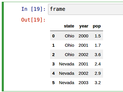
frame = pd.DataFrame(data)The resulting DataFrame will have its index assigned automatically, as with Series, and the columns are placed according to the order of the keys in data (which depends on their insertion order in the dictionary):
In [50]: frame
Out[50]:
    state  year  pop
0    Ohio  2000  1.5
1    Ohio  2001  1.7
2    Ohio  2002  3.6
3  Nevada  2001  2.4
4  Nevada  2002  2.9
5 Nevada 2003 3.2If you are using the Jupyter notebook, pandas DataFrame objects will be displayed as a more browser-friendly HTML table. See Figure 5.1 for an example.
For large DataFrames, the head method selects only the first five rows:
In [51]: frame.head()
Out[51]:
    state  year  pop
0    Ohio  2000  1.5
1    Ohio  2001  1.7
2    Ohio  2002  3.6
3  Nevada  2001  2.4
4  Nevada  2002  2.9
Similarly, tail returns the last five rows:
In [52]: frame.tail()
Out[52]:
    state  year  pop
1    Ohio  2001  1.7
2    Ohio  2002  3.6
3  Nevada  2001  2.4
4  Nevada  2002  2.9
5  Nevada  2003  3.2
If you specify a sequence of columns, the DataFrame’s columns will be arranged in that order:
In [53]: pd.DataFrame(data, columns=["year", "state", "pop"])
Out[53]:
   year   state  pop
0  2000    Ohio  1.5
1  2001    Ohio  1.7
2  2002    Ohio  3.6
3  2001  Nevada  2.4
4  2002  Nevada  2.9
5  2003  Nevada  3.2
If you pass a column that isn’t contained in the dictionary, it will appear with missing values in the result:
In [54]: frame2 = pd.DataFrame(data, columns=["year", "state", "pop", "debt"])

In [55]: frame2
Out[55]:
   year   state  pop debt
0  2000    Ohio  1.5  NaN
1  2001    Ohio  1.7  NaN
2  2002    Ohio  3.6  NaN
3  2001  Nevada  2.4  NaN
4  2002  Nevada  2.9  NaN
5  2003  Nevada  3.2  NaN

In [56]: frame2.columns
Out[56]: Index(['year', 'state', 'pop', 'debt'], dtype='object')
A column in a DataFrame can be retrieved as a Series either by dictionary-like notation or by using the dot attribute notation:
In [57]: frame2["state"]
Out[57]:
0      Ohio
1      Ohio
2      Ohio
3    Nevada
4    Nevada
5    Nevada
Name: state, dtype: object

In [58]: frame2.year
Out[58]:
0    2000
1    2001
2    2002
3    2001
4    2002
5    2003
Name: year, dtype: int64Attribute-like access (e.g., frame2.year) and tab completion of column names in IPython are provided as a convenience.
frame2[column] works for any column name, but frame2.column works only when the column name is a valid Python variable name and does not conflict with any of the method names in DataFrame. For example, if a column's name contains whitespace or symbols other than underscores, it cannot be accessed with the dot attribute method.
Note that the returned Series have the same index as the DataFrame, and their name attribute has been appropriately set.
Rows can also be retrieved by position or name with the special iloc and loc attributes (more on this later in Selection on DataFrame with loc and iloc):
In [59]: frame2.loc[1]
Out[59]:
year     2001
state    Ohio
pop       1.7
debt      NaN
Name: 1, dtype: object

In [60]: frame2.iloc[2]
Out[60]:
year     2002
state    Ohio
pop       3.6
debt      NaN
Name: 2, dtype: object
Columns can be modified by assignment. For example, the empty debt column could be assigned a scalar value or an array of values:
In [61]: frame2["debt"] = 16.5

In [62]: frame2
Out[62]:
   year   state  pop  debt
0  2000    Ohio  1.5  16.5
1  2001    Ohio  1.7  16.5
2  2002    Ohio  3.6  16.5
3  2001  Nevada  2.4  16.5
4  2002  Nevada  2.9  16.5
5  2003  Nevada  3.2  16.5

In [63]: frame2["debt"] = np.arange(6.)

In [64]: frame2
Out[64]:
   year   state  pop  debt
0  2000    Ohio  1.5   0.0
1  2001    Ohio  1.7   1.0
2  2002    Ohio  3.6   2.0
3  2001  Nevada  2.4   3.0
4  2002  Nevada  2.9   4.0
5  2003  Nevada  3.2   5.0
When you are assigning lists or arrays to a column, the value’s length must match the length of the DataFrame. If you assign a Series, its labels will be realigned exactly to the DataFrame’s index, inserting missing values in any index values not present:
In [65]: val = pd.Series([-1.2, -1.5, -1.7], index=[2, 4, 5])

In [66]: frame2["debt"] = val

In [67]: frame2
Out[67]:
   year   state  pop  debt
0  2000    Ohio  1.5   NaN
1  2001    Ohio  1.7   NaN
2  2002    Ohio  3.6  -1.2
3  2001  Nevada  2.4   NaN
4  2002  Nevada  2.9  -1.5
5  2003  Nevada  3.2  -1.7
Assigning a column that doesn’t exist will create a new column.
The del keyword will delete columns like with a dictionary. As an example, I first add a new column of Boolean values where the state column equals "Ohio":
In [68]: frame2["eastern"] = frame2["state"] == "Ohio"

In [69]: frame2
Out[69]:
   year   state  pop  debt  eastern
0  2000    Ohio  1.5   NaN     True
1  2001    Ohio  1.7   NaN     True
2  2002    Ohio  3.6  -1.2     True
3  2001  Nevada  2.4   NaN    False
4  2002  Nevada  2.9  -1.5    False
5 2003 Nevada 3.2 -1.7 FalseNew columns cannot be created with the frame2.eastern dot attribute notation.
The del method can then be used to remove this column:
In [70]: del frame2["eastern"]

In [71]: frame2.columns
Out[71]: Index(['year', 'state', 'pop', 'debt'], dtype='object')The column returned from indexing a DataFrame is a view on the underlying data, not a copy. Thus, any in-place modifications to the Series will be reflected in the DataFrame. The column can be explicitly copied with the Series’s copy method.
Another common form of data is a nested dictionary of dictionaries:
In [72]: populations = {"Ohio": {2000: 1.5, 2001: 1.7, 2002: 3.6},
   ....:                "Nevada": {2001: 2.4, 2002: 2.9}}
If the nested dictionary is passed to the DataFrame, pandas will interpret the outer dictionary keys as the columns, and the inner keys as the row indices:
In [73]: frame3 = pd.DataFrame(populations)

In [74]: frame3
Out[74]:
      Ohio  Nevada
2000   1.5     NaN
2001   1.7     2.4
2002   3.6     2.9
You can transpose the DataFrame (swap rows and columns) with similar syntax to a NumPy array:
In [75]: frame3.T
Out[75]:
        2000  2001  2002
Ohio     1.5   1.7   3.6
Nevada NaN 2.4 2.9Note that transposing discards the column data types if the columns do not all have the same data type, so transposing and then transposing back may lose the previous type information. The columns become arrays of pure Python objects in this case.
The keys in the inner dictionaries are combined to form the index in the result. This isn’t true if an explicit index is specified:
In [76]: pd.DataFrame(populations, index=[2001, 2002, 2003])
Out[76]:
      Ohio  Nevada
2001   1.7     2.4
2002   3.6     2.9
2003   NaN     NaN
Dictionaries of Series are treated in much the same way:
In [77]: pdata = {"Ohio": frame3["Ohio"][:-1],
   ....:          "Nevada": frame3["Nevada"][:2]}

In [78]: pd.DataFrame(pdata)
Out[78]:
      Ohio  Nevada
2000   1.5     NaN
2001   1.7     2.4
For a list of many of the things you can pass to the DataFrame constructor, see Table 5.1.
| Type | Notes |
|---|---|
| 2D ndarray | A matrix of data, passing optional row and column labels |
| Dictionary of arrays, lists, or tuples | Each sequence becomes a column in the DataFrame; all sequences must be the same length |
| NumPy structured/record array | Treated as the “dictionary of arrays” case |
| Dictionary of Series | Each value becomes a column; indexes from each Series are unioned together to form the result’s row index if no explicit index is passed |
| Dictionary of dictionaries | Each inner dictionary becomes a column; keys are unioned to form the row index as in the “dictionary of Series” case |
| List of dictionaries or Series | Each item becomes a row in the DataFrame; unions of dictionary keys or Series indexes become the DataFrame’s column labels |
| List of lists or tuples | Treated as the “2D ndarray” case |
| Another DataFrame | The DataFrame’s indexes are used unless different ones are passed |
| NumPy MaskedArray | Like the “2D ndarray” case except masked values are missing in the DataFrame result |
If a DataFrame’s index and columns have their name attributes set, these will also be displayed:
In [79]: frame3.index.name = "year"

In [80]: frame3.columns.name = "state"

In [81]: frame3
Out[81]:
state  Ohio  Nevada
year
2000    1.5     NaN
2001    1.7     2.4
2002    3.6     2.9
Unlike Series, DataFrame does not have a name attribute. DataFrame's to_numpy method returns the data contained in the DataFrame as a two-dimensional ndarray:
In [82]: frame3.to_numpy()
Out[82]:
array([[1.5, nan],
       [1.7, 2.4],
       [3.6, 2.9]])
If the DataFrame’s columns are different data types, the data type of the returned array will be chosen to accommodate all of the columns:
In [83]: frame2.to_numpy()
Out[83]:
array([[2000, 'Ohio', 1.5, nan],
       [2001, 'Ohio', 1.7, nan],
       [2002, 'Ohio', 3.6, -1.2],
       [2001, 'Nevada', 2.4, nan],
       [2002, 'Nevada', 2.9, -1.5],
       [2003, 'Nevada', 3.2, -1.7]], dtype=object)
Index Objects
pandas’s Index objects are responsible for holding the axis labels (including a DataFrame's column names) and other metadata (like the axis name or names). Any array or other sequence of labels you use when constructing a Series or DataFrame is internally converted to an Index:
In [84]: obj = pd.Series(np.arange(3), index=["a", "b", "c"])

In [85]: index = obj.index

In [86]: index
Out[86]: Index(['a', 'b', 'c'], dtype='object')

In [87]: index[1:]
Out[87]: Index(['b', 'c'], dtype='object')
Index objects are immutable and thus can’t be modified by the user:
index[1] = "d" # TypeErrorImmutability makes it safer to share Index objects among data structures:
In [88]: labels = pd.Index(np.arange(3))

In [89]: labels
Out[89]: Index([0, 1, 2], dtype='int64')

In [90]: obj2 = pd.Series([1.5, -2.5, 0], index=labels)

In [91]: obj2
Out[91]:
0    1.5
1   -2.5
2    0.0
dtype: float64

In [92]: obj2.index is labels
Out[92]: TrueSome users will not often take advantage of the capabilities provided by an Index, but because some operations will yield results containing indexed data, it's important to understand how they work.
In addition to being array-like, an Index also behaves like a fixed-size set:
In [93]: frame3
Out[93]:
state  Ohio  Nevada
year
2000    1.5     NaN
2001    1.7     2.4
2002    3.6     2.9

In [94]: frame3.columns
Out[94]: Index(['Ohio', 'Nevada'], dtype='object', name='state')

In [95]: "Ohio" in frame3.columns
Out[95]: True

In [96]: 2003 in frame3.index
Out[96]: False
Unlike Python sets, a pandas Index can contain duplicate labels:
In [97]: pd.Index(["foo", "foo", "bar", "bar"])
Out[97]: Index(['foo', 'foo', 'bar', 'bar'], dtype='object')
Selections with duplicate labels will select all occurrences of that label.
Each Index has a number of methods and properties for set logic, which answer other common questions about the data it contains. Some useful ones are summarized in Table 5.2.
| Method/Property | Description |
|---|---|
append() |
Concatenate with additional Index objects, producing a new Index |
difference() |
Compute set difference as an Index |
intersection() |
Compute set intersection |
union() |
Compute set union |
isin() |
Compute Boolean array indicating whether each value is contained in the passed collection |
delete() |
Compute new Index with element at Index i deleted |
drop() |
Compute new Index by deleting passed values |
insert() |
Compute new Index by inserting element at Index i |
is_monotonic |
Returns True if each element is greater than or equal to the previous element |
is_unique |
Returns True if the Index has no duplicate values |
unique() |
Compute the array of unique values in the Index |
5.2 Essential Functionality
This section will walk you through the fundamental mechanics of interacting with the data contained in a Series or DataFrame. In the chapters to come, we will delve more deeply into data analysis and manipulation topics using pandas. This book is not intended to serve as exhaustive documentation for the pandas library; instead, we'll focus on familiarizing you with heavily used features, leaving the less common (i.e., more esoteric) things for you to learn more about by reading the online pandas documentation.
Reindexing
An important method on pandas objects is reindex, which means to create a new object with the values rearranged to align with the new index. Consider an example:
In [98]: obj = pd.Series([4.5, 7.2, -5.3, 3.6], index=["d", "b", "a", "c"])

In [99]: obj
Out[99]:
d    4.5
b    7.2
a   -5.3
c    3.6
dtype: float64
Calling reindex on this Series rearranges the data according to the new index, introducing missing values if any index values were not already present:
In [100]: obj2 = obj.reindex(["a", "b", "c", "d", "e"])

In [101]: obj2
Out[101]:
a   -5.3
b    7.2
c    3.6
d    4.5
e    NaN
dtype: float64
For ordered data like time series, you may want to do some interpolation or filling of values when reindexing. The method option allows us to do this, using a method such as ffill, which forward-fills the values:
In [102]: obj3 = pd.Series(["blue", "purple", "yellow"], index=[0, 2, 4])

In [103]: obj3
Out[103]:
0      blue
2    purple
4    yellow
dtype: object

In [104]: obj3.reindex(np.arange(6), method="ffill")
Out[104]:
0      blue
1      blue
2    purple
3    purple
4    yellow
5    yellow
dtype: object
With DataFrame, reindex can alter the (row) index, columns, or both. When passed only a sequence, it reindexes the rows in the result:
In [105]: frame = pd.DataFrame(np.arange(9).reshape((3, 3)),
   .....:                      index=["a", "c", "d"],
   .....:                      columns=["Ohio", "Texas", "California"])

In [106]: frame
Out[106]:
   Ohio  Texas  California
a     0      1           2
c     3      4           5
d     6      7           8

In [107]: frame2 = frame.reindex(index=["a", "b", "c", "d"])

In [108]: frame2
Out[108]:
   Ohio  Texas  California
a   0.0    1.0         2.0
b   NaN    NaN         NaN
c   3.0    4.0         5.0
d   6.0    7.0         8.0
The columns can be reindexed with the columns keyword:
In [109]: states = ["Texas", "Utah", "California"]

In [110]: frame.reindex(columns=states)
Out[110]:
   Texas  Utah  California
a      1   NaN           2
c      4   NaN           5
d      7   NaN           8
Because "Ohio" was not in states, the data for that column is dropped from the result.
Another way to reindex a particular axis is to pass the new axis labels as a positional argument and then specify the axis to reindex with the axis keyword:
In [111]: frame.reindex(states, axis="columns")
Out[111]:
   Texas  Utah  California
a      1   NaN           2
c      4   NaN           5
d      7   NaN           8
See Table 5.3 for more about the arguments to reindex.
| Argument | Description |
|---|---|
labels |
New sequence to use as an index. Can be Index instance or any other sequence-like Python data structure. An Index will be used exactly as is without any copying. |
index |
Use the passed sequence as the new index labels. |
columns |
Use the passed sequence as the new column labels. |
axis |
The axis to reindex, whether "index" (rows) or "columns". The default is "index". You can alternately do reindex(index=new_labels) or reindex(columns=new_labels). |
method |
Interpolation (fill) method; "ffill" fills forward, while "bfill" fills backward. |
fill_value |
Substitute value to use when introducing missing data by reindexing. Use fill_value="missing" (the default behavior) when you want absent labels to have null values in the result. |
limit |
When forward filling or backfilling, the maximum size gap (in number of elements) to fill. |
tolerance |
When forward filling or backfilling, the maximum size gap (in absolute numeric distance) to fill for inexact matches. |
level |
Match simple Index on level of MultiIndex; otherwise select subset of. |
copy |
If True, always copy underlying data even if the new index is equivalent to the old index; if False, do not copy the data when the indexes are equivalent. |
As we'll explore later in Selection on DataFrame with loc and iloc, you can also reindex by using the loc operator, and many users prefer to always do it this way. This works only if all of the new index labels already exist in the DataFrame (whereas reindex will insert missing data for new labels):
In [112]: frame.loc[["a", "d", "c"], ["California", "Texas"]]
Out[112]:
   California  Texas
a           2      1
d           8      7
c           5      4
Dropping Entries from an Axis
Dropping one or more entries from an axis is simple if you already have an index array or list without those entries, since you can use the reindex method or .loc-based indexing. As that can require a bit of munging and set logic, the drop method will return a new object with the indicated value or values deleted from an axis:
In [113]: obj = pd.Series(np.arange(5.), index=["a", "b", "c", "d", "e"])

In [114]: obj
Out[114]:
a    0.0
b    1.0
c    2.0
d    3.0
e    4.0
dtype: float64

In [115]: new_obj = obj.drop("c")

In [116]: new_obj
Out[116]:
a    0.0
b    1.0
d    3.0
e    4.0
dtype: float64

In [117]: obj.drop(["d", "c"])
Out[117]:
a    0.0
b    1.0
e    4.0
dtype: float64
With DataFrame, index values can be deleted from either axis. To illustrate this, we first create an example DataFrame:
In [118]: data = pd.DataFrame(np.arange(16).reshape((4, 4)),
   .....:                     index=["Ohio", "Colorado", "Utah", "New York"],
   .....:                     columns=["one", "two", "three", "four"])

In [119]: data
Out[119]:
          one  two  three  four
Ohio        0    1      2     3
Colorado    4    5      6     7
Utah        8    9     10    11
New York   12   13     14    15
Calling drop with a sequence of labels will drop values from the row labels (axis 0):
In [120]: data.drop(index=["Colorado", "Ohio"])
Out[120]:
          one  two  three  four
Utah        8    9     10    11
New York   12   13     14    15
To drop labels from the columns, instead use the columns keyword:
In [121]: data.drop(columns=["two"])
Out[121]:
          one  three  four
Ohio        0      2     3
Colorado    4      6     7
Utah        8     10    11
New York   12     14    15
You can also drop values from the columns by passing axis=1 (which is like NumPy) or axis="columns":
In [122]: data.drop("two", axis=1)
Out[122]:
          one  three  four
Ohio        0      2     3
Colorado    4      6     7
Utah        8     10    11
New York   12     14    15

In [123]: data.drop(["two", "four"], axis="columns")
Out[123]:
          one  three
Ohio        0      2
Colorado    4      6
Utah        8     10
New York   12     14
Indexing, Selection, and Filtering
Series indexing (obj[...]) works analogously to NumPy array indexing, except you can use the Series’s index values instead of only integers. Here are some examples of this:
In [124]: obj = pd.Series(np.arange(4.), index=["a", "b", "c", "d"])

In [125]: obj
Out[125]:
a    0.0
b    1.0
c    2.0
d    3.0
dtype: float64

In [126]: obj["b"]
Out[126]: 1.0

In [127]: obj[1]
Out[127]: 1.0

In [128]: obj[2:4]
Out[128]:
c    2.0
d    3.0
dtype: float64

In [129]: obj[["b", "a", "d"]]
Out[129]:
b    1.0
a    0.0
d    3.0
dtype: float64

In [130]: obj[[1, 3]]
Out[130]:
b    1.0
d    3.0
dtype: float64

In [131]: obj[obj < 2]
Out[131]:
a    0.0
b    1.0
dtype: float64
While you can select data by label this way, the preferred way to select index values is with the special loc operator:
In [132]: obj.loc[["b", "a", "d"]]
Out[132]:
b    1.0
a    0.0
d    3.0
dtype: float64
The reason to prefer loc is because of the different treatment of integers when indexing with []. Regular []-based indexing will treat integers as labels if the index contains integers, so the behavior differs depending on the data type of the index. For example:
In [133]: obj1 = pd.Series([1, 2, 3], index=[2, 0, 1])

In [134]: obj2 = pd.Series([1, 2, 3], index=["a", "b", "c"])

In [135]: obj1
Out[135]:
2    1
0    2
1    3
dtype: int64

In [136]: obj2
Out[136]:
a    1
b    2
c    3
dtype: int64

In [137]: obj1[[0, 1, 2]]
Out[137]:
0    2
1    3
2    1
dtype: int64

In [138]: obj2[[0, 1, 2]]
Out[138]:
a    1
b    2
c    3
dtype: int64
When using loc, the expression obj.loc[[0, 1, 2]] will fail when the index does not contain integers:
In [134]: obj2.loc[[0, 1]]
---------------------------------------------------------------------------
KeyError                                  Traceback (most recent call last)
/tmp/ipykernel_804589/4185657903.py in <module>
----> 1 obj2.loc[[0, 1]]

^ LONG EXCEPTION ABBREVIATED ^

KeyError: "None of [Int64Index([0, 1], dtype="int64")] are in the [index]"
Since loc operator indexes exclusively with labels, there is also an iloc operator that indexes exclusively with integers to work consistently whether or not the index contains integers:
In [139]: obj1.iloc[[0, 1, 2]]
Out[139]:
2    1
0    2
1    3
dtype: int64

In [140]: obj2.iloc[[0, 1, 2]]
Out[140]:
a    1
b    2
c    3
dtype: int64You can also slice with labels, but it works differently from normal Python slicing in that the endpoint is inclusive:
In [141]: obj2.loc["b":"c"]
Out[141]:
b    2
c    3
dtype: int64
Assigning values using these methods modifies the corresponding section of the Series:
In [142]: obj2.loc["b":"c"] = 5

In [143]: obj2
Out[143]:
a    1
b    5
c    5
dtype: int64It can be a common newbie error to try to call loc or iloc like functions rather than "indexing into" them with square brackets. The square bracket notation is used to enable slice operations and to allow for indexing on multiple axes with DataFrame objects.
Indexing into a DataFrame retrieves one or more columns either with a single value or sequence:
In [144]: data = pd.DataFrame(np.arange(16).reshape((4, 4)),
   .....:                     index=["Ohio", "Colorado", "Utah", "New York"],
   .....:                     columns=["one", "two", "three", "four"])

In [145]: data
Out[145]:
          one  two  three  four
Ohio        0    1      2     3
Colorado    4    5      6     7
Utah        8    9     10    11
New York   12   13     14    15

In [146]: data["two"]
Out[146]:
Ohio         1
Colorado     5
Utah         9
New York    13
Name: two, dtype: int64

In [147]: data[["three", "one"]]
Out[147]:
          three  one
Ohio          2    0
Colorado      6    4
Utah         10    8
New York     14   12
Indexing like this has a few special cases. The first is slicing or selecting data with a Boolean array:
In [148]: data[:2]
Out[148]:
          one  two  three  four
Ohio        0    1      2     3
Colorado    4    5      6     7

In [149]: data[data["three"] > 5]
Out[149]:
          one  two  three  four
Colorado    4    5      6     7
Utah        8    9     10    11
New York   12   13     14    15
The row selection syntax data[:2] is provided as a convenience. Passing a single element or a list to the [] operator selects columns.
Another use case is indexing with a Boolean DataFrame, such as one produced by a scalar comparison. Consider a DataFrame with all Boolean values produced by comparing with a scalar value:
In [150]: data < 5
Out[150]:
            one    two  three   four
Ohio       True   True   True   True
Colorado   True  False  False  False
Utah      False  False  False  False
New York  False  False  False  False
We can use this DataFrame to assign the value 0 to each location with the value True, like so:
In [151]: data[data < 5] = 0

In [152]: data
Out[152]:
          one  two  three  four
Ohio        0    0      0     0
Colorado    0    5      6     7
Utah        8    9     10    11
New York   12   13     14    15
Selection on DataFrame with loc and iloc
Like Series, DataFrame has special attributes loc and iloc for label-based and integer-based indexing, respectively. Since DataFrame is two-dimensional, you can select a subset of the rows and columns with NumPy-like notation using either axis labels (loc) or integers (iloc).
As a first example, let's select a single row by label:
In [153]: data
Out[153]:
          one  two  three  four
Ohio        0    0      0     0
Colorado    0    5      6     7
Utah        8    9     10    11
New York   12   13     14    15

In [154]: data.loc["Colorado"]
Out[154]:
one      0
two      5
three    6
four     7
Name: Colorado, dtype: int64
The result of selecting a single row is a Series with an index that contains the DataFrame's column labels. To select multiple roles, creating a new DataFrame, pass a sequence of labels:
In [155]: data.loc[["Colorado", "New York"]]
Out[155]:
          one  two  three  four
Colorado    0    5      6     7
New York   12   13     14    15
You can combine both row and column selection in loc by separating the selections with a comma:
In [156]: data.loc["Colorado", ["two", "three"]]
Out[156]:
two      5
three    6
Name: Colorado, dtype: int64
We'll then perform some similar selections with integers using iloc:
In [157]: data.iloc[2]
Out[157]:
one       8
two       9
three    10
four     11
Name: Utah, dtype: int64

In [158]: data.iloc[[2, 1]]
Out[158]:
          one  two  three  four
Utah        8    9     10    11
Colorado    0    5      6     7

In [159]: data.iloc[2, [3, 0, 1]]
Out[159]:
four    11
one      8
two      9
Name: Utah, dtype: int64

In [160]: data.iloc[[1, 2], [3, 0, 1]]
Out[160]:
          four  one  two
Colorado     7    0    5
Utah        11    8    9
Both indexing functions work with slices in addition to single labels or lists of labels:
In [161]: data.loc[:"Utah", "two"]
Out[161]:
Ohio        0
Colorado    5
Utah        9
Name: two, dtype: int64

In [162]: data.iloc[:, :3][data.three > 5]
Out[162]:
          one  two  three
Colorado    0    5      6
Utah        8    9     10
New York   12   13     14
Boolean arrays can be used with loc but not iloc:
In [163]: data.loc[data.three >= 2]
Out[163]:
          one  two  three  four
Colorado    0    5      6     7
Utah        8    9     10    11
New York   12   13     14    15
There are many ways to select and rearrange the data contained in a pandas object. For DataFrame, Table 5.4 provides a short summary of many of them. As you will see later, there are a number of additional options for working with hierarchical indexes.
| Type | Notes |
|---|---|
df[column] |
Select single column or sequence of columns from the DataFrame; special case conveniences: Boolean array (filter rows), slice (slice rows), or Boolean DataFrame (set values based on some criterion) |
df.loc[rows] |
Select single row or subset of rows from the DataFrame by label |
df.loc[:, cols] |
Select single column or subset of columns by label |
df.loc[rows, cols] |
Select both row(s) and column(s) by label |
df.iloc[rows] |
Select single row or subset of rows from the DataFrame by integer position |
df.iloc[:, cols] |
Select single column or subset of columns by integer position |
df.iloc[rows, cols] |
Select both row(s) and column(s) by integer position |
df.at[row, col] |
Select a single scalar value by row and column label |
df.iat[row, col] |
Select a single scalar value by row and column position (integers) |
reindex method |
Select either rows or columns by labels |
Integer indexing pitfalls
Working with pandas objects indexed by integers can be a stumbling block for new users since they work differently from built-in Python data structures like lists and tuples. For example, you might not expect the following code to generate an error:
In [164]: ser = pd.Series(np.arange(3.))

In [165]: ser
Out[165]:
0    0.0
1    1.0
2    2.0
dtype: float64

In [166]: ser[-1]
---------------------------------------------------------------------------
ValueError                                Traceback (most recent call last)
~/miniforge-x86/envs/book-env/lib/python3.10/site-packages/pandas/core/indexes/ra
nge.py in get_loc(self, key)
    344             try:
--> 345                 return self._range.index(new_key)
    346             except ValueError as err:
ValueError: -1 is not in range
The above exception was the direct cause of the following exception:
KeyError                                  Traceback (most recent call last)
<ipython-input-166-44969a759c20> in <module>
----> 1 ser[-1]
~/miniforge-x86/envs/book-env/lib/python3.10/site-packages/pandas/core/series.py
in __getitem__(self, key)
   1010
   1011         elif key_is_scalar:
-> 1012             return self._get_value(key)
   1013
   1014         if is_hashable(key):
~/miniforge-x86/envs/book-env/lib/python3.10/site-packages/pandas/core/series.py
in _get_value(self, label, takeable)
   1119
   1120         # Similar to Index.get_value, but we do not fall back to position
al
-> 1121         loc = self.index.get_loc(label)
   1122
   1123         if is_integer(loc):
~/miniforge-x86/envs/book-env/lib/python3.10/site-packages/pandas/core/indexes/ra
nge.py in get_loc(self, key)
    345                 return self._range.index(new_key)
    346             except ValueError as err:
--> 347                 raise KeyError(key) from err
    348         self._check_indexing_error(key)
    349         raise KeyError(key)
KeyError: -1
In this case, pandas could “fall back” on integer indexing, but it is difficult to do this in general without introducing subtle bugs into the user code. Here we have an index containing 0, 1, and 2, but pandas does not want to guess what the user wants (label-based indexing or position-based):
In [167]: ser
Out[167]:
0    0.0
1    1.0
2    2.0
dtype: float64
On the other hand, with a noninteger index, there is no such ambiguity:
In [168]: ser2 = pd.Series(np.arange(3.), index=["a", "b", "c"])

In [169]: ser2[-1]
Out[169]: 2.0
If you have an axis index containing integers, data selection will always be label oriented. As I said above, if you use loc (for labels) or iloc (for integers) you will get exactly what you want:
In [170]: ser.iloc[-1]
Out[170]: 2.0
On the other hand, slicing with integers is always integer oriented:
In [171]: ser[:2]
Out[171]:
0    0.0
1    1.0
dtype: float64
As a result of these pitfalls, it is best to always prefer indexing with loc and iloc to avoid ambiguity.
Pitfalls with chained indexing
In the previous section we looked at how you can do flexible selections on a DataFrame using loc and iloc. These indexing attributes can also be used to modify DataFrame objects in place, but doing so requires some care.
For example, in the example DataFrame above, we can assign to a column or row by label or integer position:
In [172]: data.loc[:, "one"] = 1

In [173]: data
Out[173]:
          one  two  three  four
Ohio        1    0      0     0
Colorado    1    5      6     7
Utah        1    9     10    11
New York    1   13     14    15

In [174]: data.iloc[2] = 5

In [175]: data
Out[175]:
          one  two  three  four
Ohio        1    0      0     0
Colorado    1    5      6     7
Utah        5    5      5     5
New York    1   13     14    15

In [176]: data.loc[data["four"] > 5] = 3

In [177]: data
Out[177]:
          one  two  three  four
Ohio        1    0      0     0
Colorado    3    3      3     3
Utah        5    5      5     5
New York    3    3      3     3
A common gotcha for new pandas users is to chain selections when assigning, like this:
In [177]: data.loc[data.three == 5]["three"] = 6
<ipython-input-11-0ed1cf2155d5>:1: SettingWithCopyWarning:
A value is trying to be set on a copy of a slice from a DataFrame.
Try using .loc[row_indexer,col_indexer] = value instead
Depending on the data contents, this may print a special SettingWithCopyWarning, which warns you that you are trying to modify a temporary value (the nonempty result of data.loc[data.three == 5]) instead of the original DataFrame data, which might be what you were intending. Here, data was unmodified:
In [179]: data
Out[179]:
          one  two  three  four
Ohio        1    0      0     0
Colorado    3    3      3     3
Utah        5    5      5     5
New York    3    3      3     3
In these scenarios, the fix is to rewrite the chained assignment to use a single loc operation:
In [180]: data.loc[data.three == 5, "three"] = 6

In [181]: data
Out[181]:
          one  two  three  four
Ohio        1    0      0     0
Colorado    3    3      3     3
Utah        5    5      6     5
New York    3    3      3     3
A good rule of thumb is to avoid chained indexing when doing assignments. There are other cases where pandas will generate SettingWithCopyWarning that have to do with chained indexing. I refer you to this topic in the online pandas documentation.
Arithmetic and Data Alignment
pandas can make it much simpler to work with objects that have different indexes. For example, when you add objects, if any index pairs are not the same, the respective index in the result will be the union of the index pairs. Let’s look at an example:
In [182]: s1 = pd.Series([7.3, -2.5, 3.4, 1.5], index=["a", "c", "d", "e"])

In [183]: s2 = pd.Series([-2.1, 3.6, -1.5, 4, 3.1],
   .....:                index=["a", "c", "e", "f", "g"])

In [184]: s1
Out[184]:
a    7.3
c   -2.5
d    3.4
e    1.5
dtype: float64

In [185]: s2
Out[185]:
a   -2.1
c    3.6
e   -1.5
f    4.0
g    3.1
dtype: float64
Adding these yields:
In [186]: s1 + s2
Out[186]:
a    5.2
c    1.1
d    NaN
e    0.0
f    NaN
g    NaN
dtype: float64
The internal data alignment introduces missing values in the label locations that don’t overlap. Missing values will then propagate in further arithmetic computations.
In the case of DataFrame, alignment is performed on both rows and columns:
In [187]: df1 = pd.DataFrame(np.arange(9.).reshape((3, 3)), columns=list("bcd"),
   .....:                    index=["Ohio", "Texas", "Colorado"])

In [188]: df2 = pd.DataFrame(np.arange(12.).reshape((4, 3)), columns=list("bde"),
   .....:                    index=["Utah", "Ohio", "Texas", "Oregon"])

In [189]: df1
Out[189]:
            b    c    d
Ohio      0.0  1.0  2.0
Texas     3.0  4.0  5.0
Colorado  6.0  7.0  8.0

In [190]: df2
Out[190]:
          b     d     e
Utah    0.0   1.0   2.0
Ohio    3.0   4.0   5.0
Texas   6.0   7.0   8.0
Oregon  9.0  10.0  11.0
Adding these returns a DataFrame with index and columns that are the unions of the ones in each DataFrame:
In [191]: df1 + df2
Out[191]:
            b   c     d   e
Colorado  NaN NaN   NaN NaN
Ohio      3.0 NaN   6.0 NaN
Oregon    NaN NaN   NaN NaN
Texas     9.0 NaN  12.0 NaN
Utah      NaN NaN   NaN NaN
Since the "c" and "e" columns are not found in both DataFrame objects, they appear as missing in the result. The same holds for the rows with labels that are not common to both objects.
If you add DataFrame objects with no column or row labels in common, the result will contain all nulls:
In [192]: df1 = pd.DataFrame({"A": [1, 2]})

In [193]: df2 = pd.DataFrame({"B": [3, 4]})

In [194]: df1
Out[194]:
   A
0  1
1  2

In [195]: df2
Out[195]:
   B
0  3
1  4

In [196]: df1 + df2
Out[196]:
    A   B
0 NaN NaN
1 NaN NaN
Arithmetic methods with fill values
In arithmetic operations between differently indexed objects, you might want to fill with a special value, like 0, when an axis label is found in one object but not the other. Here is an example where we set a particular value to NA (null) by assigning np.nan to it:
In [197]: df1 = pd.DataFrame(np.arange(12.).reshape((3, 4)),
   .....:                    columns=list("abcd"))

In [198]: df2 = pd.DataFrame(np.arange(20.).reshape((4, 5)),
   .....:                    columns=list("abcde"))

In [199]: df2.loc[1, "b"] = np.nan

In [200]: df1
Out[200]:
     a    b     c     d
0  0.0  1.0   2.0   3.0
1  4.0  5.0   6.0   7.0
2  8.0  9.0  10.0  11.0

In [201]: df2
Out[201]:
      a     b     c     d     e
0   0.0   1.0   2.0   3.0   4.0
1   5.0   NaN   7.0   8.0   9.0
2  10.0  11.0  12.0  13.0  14.0
3  15.0  16.0  17.0  18.0  19.0
Adding these results in missing values in the locations that don’t overlap:
In [202]: df1 + df2
Out[202]:
      a     b     c     d   e
0   0.0   2.0   4.0   6.0 NaN
1   9.0   NaN  13.0  15.0 NaN
2  18.0  20.0  22.0  24.0 NaN
3   NaN   NaN   NaN   NaN NaN
Using the add method on df1, I pass df2 and an argument to fill_value, which substitutes the passed value for any missing values in the operation:
In [203]: df1.add(df2, fill_value=0)
Out[203]:
      a     b     c     d     e
0   0.0   2.0   4.0   6.0   4.0
1   9.0   5.0  13.0  15.0   9.0
2  18.0  20.0  22.0  24.0  14.0
3  15.0  16.0  17.0  18.0  19.0
See Table 5.5 for a listing of Series and DataFrame methods for arithmetic. Each has a counterpart, starting with the letter r, that has arguments reversed. So these two statements are equivalent:
In [204]: 1 / df1
Out[204]:
       a         b         c         d
0    inf  1.000000  0.500000  0.333333
1  0.250  0.200000  0.166667  0.142857
2  0.125  0.111111  0.100000  0.090909

In [205]: df1.rdiv(1)
Out[205]:
       a         b         c         d
0    inf  1.000000  0.500000  0.333333
1  0.250  0.200000  0.166667  0.142857
2  0.125  0.111111  0.100000  0.090909
Relatedly, when reindexing a Series or DataFrame, you can also specify a different fill value:
In [206]: df1.reindex(columns=df2.columns, fill_value=0)
Out[206]:
     a    b     c     d  e
0  0.0  1.0   2.0   3.0  0
1  4.0  5.0   6.0   7.0  0
2 8.0 9.0 10.0 11.0 0| Method | Description |
|---|---|
add, radd |
Methods for addition (+) |
sub, rsub |
Methods for subtraction (-) |
div, rdiv |
Methods for division (/) |
floordiv, rfloordiv |
Methods for floor division (//) |
mul, rmul |
Methods for multiplication (*) |
pow, rpow |
Methods for exponentiation (**) |
Operations between DataFrame and Series
As with NumPy arrays of different dimensions, arithmetic between DataFrame and Series is also defined. First, as a motivating example, consider the difference between a two-dimensional array and one of its rows:
In [207]: arr = np.arange(12.).reshape((3, 4))

In [208]: arr
Out[208]:
array([[ 0.,  1.,  2.,  3.],
       [ 4.,  5.,  6.,  7.],
       [ 8.,  9., 10., 11.]])

In [209]: arr[0]
Out[209]: array([0., 1., 2., 3.])

In [210]: arr - arr[0]
Out[210]:
array([[0., 0., 0., 0.],
       [4., 4., 4., 4.],
       [8., 8., 8., 8.]])
When we subtract arr[0] from arr, the subtraction is performed once for each row. This is referred to as broadcasting and is explained in more detail as it relates to general NumPy arrays in Appendix A: Advanced NumPy. Operations between a DataFrame and a Series are similar:
In [211]: frame = pd.DataFrame(np.arange(12.).reshape((4, 3)),
   .....:                      columns=list("bde"),
   .....:                      index=["Utah", "Ohio", "Texas", "Oregon"])

In [212]: series = frame.iloc[0]

In [213]: frame
Out[213]:
          b     d     e
Utah    0.0   1.0   2.0
Ohio    3.0   4.0   5.0
Texas   6.0   7.0   8.0
Oregon  9.0  10.0  11.0

In [214]: series
Out[214]:
b    0.0
d    1.0
e    2.0
Name: Utah, dtype: float64
By default, arithmetic between DataFrame and Series matches the index of the Series on the columns of the DataFrame, broadcasting down the rows:
In [215]: frame - series
Out[215]:
          b    d    e
Utah    0.0  0.0  0.0
Ohio    3.0  3.0  3.0
Texas   6.0  6.0  6.0
Oregon  9.0  9.0  9.0
If an index value is not found in either the DataFrame’s columns or the Series’s index, the objects will be reindexed to form the union:
In [216]: series2 = pd.Series(np.arange(3), index=["b", "e", "f"])

In [217]: series2
Out[217]:
b    0
e    1
f    2
dtype: int64

In [218]: frame + series2
Out[218]:
          b   d     e   f
Utah    0.0 NaN   3.0 NaN
Ohio    3.0 NaN   6.0 NaN
Texas   6.0 NaN   9.0 NaN
Oregon  9.0 NaN  12.0 NaN
If you want to instead broadcast over the columns, matching on the rows, you have to use one of the arithmetic methods and specify to match over the index. For example:
In [219]: series3 = frame["d"]

In [220]: frame
Out[220]:
          b     d     e
Utah    0.0   1.0   2.0
Ohio    3.0   4.0   5.0
Texas   6.0   7.0   8.0
Oregon  9.0  10.0  11.0

In [221]: series3
Out[221]:
Utah       1.0
Ohio       4.0
Texas      7.0
Oregon    10.0
Name: d, dtype: float64

In [222]: frame.sub(series3, axis="index")
Out[222]:
          b    d    e
Utah   -1.0  0.0  1.0
Ohio   -1.0  0.0  1.0
Texas  -1.0  0.0  1.0
Oregon -1.0  0.0  1.0
The axis that you pass is the axis to match on. In this case we mean to match on the DataFrame’s row index (axis="index") and broadcast across the columns.
Function Application and Mapping
NumPy ufuncs (element-wise array methods) also work with pandas objects:
In [223]: frame = pd.DataFrame(np.random.standard_normal((4, 3)),
   .....:                      columns=list("bde"),
   .....:                      index=["Utah", "Ohio", "Texas", "Oregon"])

In [224]: frame
Out[224]:
               b         d         e
Utah   -0.204708  0.478943 -0.519439
Ohio   -0.555730  1.965781  1.393406
Texas   0.092908  0.281746  0.769023
Oregon  1.246435  1.007189 -1.296221

In [225]: np.abs(frame)
Out[225]:
               b         d         e
Utah    0.204708  0.478943  0.519439
Ohio    0.555730  1.965781  1.393406
Texas   0.092908  0.281746  0.769023
Oregon  1.246435  1.007189  1.296221
Another frequent operation is applying a function on one-dimensional arrays to each column or row. DataFrame’s apply method does exactly this:
In [226]: def f1(x):
   .....:     return x.max() - x.min()

In [227]: frame.apply(f1)
Out[227]:
b    1.802165
d    1.684034
e    2.689627
dtype: float64
Here the function f, which computes the difference between the maximum and minimum of a Series, is invoked once on each column in frame. The result is a Series having the columns of frame as its index.
If you pass axis="columns" to apply, the function will be invoked once per row instead. A helpful way to think about this is as "apply across the columns":
In [228]: frame.apply(f1, axis="columns")
Out[228]:
Utah      0.998382
Ohio      2.521511
Texas     0.676115
Oregon    2.542656
dtype: float64
Many of the most common array statistics (like sum and mean) are DataFrame methods, so using apply is not necessary.
The function passed to apply need not return a scalar value; it can also return a Series with multiple values:
In [229]: def f2(x):
   .....:     return pd.Series([x.min(), x.max()], index=["min", "max"])

In [230]: frame.apply(f2)
Out[230]:
            b         d         e
min -0.555730  0.281746 -1.296221
max  1.246435  1.965781  1.393406
Element-wise Python functions can be used, too. Suppose you wanted to compute a formatted string from each floating-point value in frame. You can do this with applymap:
In [231]: def my_format(x):
   .....:     return f"{x:.2f}"

In [232]: frame.applymap(my_format)
Out[232]:
            b     d      e
Utah    -0.20  0.48  -0.52
Ohio    -0.56  1.97   1.39
Texas    0.09  0.28   0.77
Oregon   1.25  1.01  -1.30
The reason for the name applymap is that Series has a map method for applying an element-wise function:
In [233]: frame["e"].map(my_format)
Out[233]:
Utah      -0.52
Ohio       1.39
Texas      0.77
Oregon    -1.30
Name: e, dtype: object
Sorting and Ranking
Sorting a dataset by some criterion is another important built-in operation. To sort lexicographically by row or column label, use the sort_index method, which returns a new, sorted object:
In [234]: obj = pd.Series(np.arange(4), index=["d", "a", "b", "c"])

In [235]: obj
Out[235]:
d    0
a    1
b    2
c    3
dtype: int64

In [236]: obj.sort_index()
Out[236]:
a    1
b    2
c    3
d    0
dtype: int64
With a DataFrame, you can sort by index on either axis:
In [237]: frame = pd.DataFrame(np.arange(8).reshape((2, 4)),
   .....:                      index=["three", "one"],
   .....:                      columns=["d", "a", "b", "c"])

In [238]: frame
Out[238]:
       d  a  b  c
three  0  1  2  3
one    4  5  6  7

In [239]: frame.sort_index()
Out[239]:
       d  a  b  c
one    4  5  6  7
three  0  1  2  3

In [240]: frame.sort_index(axis="columns")
Out[240]:
       a  b  c  d
three  1  2  3  0
one    5  6  7  4
The data is sorted in ascending order by default but can be sorted in descending order, too:
In [241]: frame.sort_index(axis="columns", ascending=False)
Out[241]:
       d  c  b  a
three  0  3  2  1
one    4  7  6  5
To sort a Series by its values, use its sort_values method:
In [242]: obj = pd.Series([4, 7, -3, 2])

In [243]: obj.sort_values()
Out[243]:
2   -3
3    2
0    4
1    7
dtype: int64
Any missing values are sorted to the end of the Series by default:
In [244]: obj = pd.Series([4, np.nan, 7, np.nan, -3, 2])

In [245]: obj.sort_values()
Out[245]:
4   -3.0
5    2.0
0    4.0
2    7.0
1    NaN
3    NaN
dtype: float64
Missing values can be sorted to the start instead by using the na_position option:
In [246]: obj.sort_values(na_position="first")
Out[246]:
1    NaN
3    NaN
4   -3.0
5    2.0
0    4.0
2    7.0
dtype: float64
When sorting a DataFrame, you can use the data in one or more columns as the sort keys. To do so, pass one or more column names to sort_values:
In [247]: frame = pd.DataFrame({"b": [4, 7, -3, 2], "a": [0, 1, 0, 1]})

In [248]: frame
Out[248]:
   b  a
0  4  0
1  7  1
2 -3  0
3  2  1

In [249]: frame.sort_values("b")
Out[249]:
   b  a
2 -3  0
3  2  1
0  4  0
1  7  1
To sort by multiple columns, pass a list of names:
In [250]: frame.sort_values(["a", "b"])
Out[250]:
   b  a
2 -3  0
0  4  0
3  2  1
1  7  1
Ranking assigns ranks from one through the number of valid data points in an array, starting from the lowest value. The rank methods for Series and DataFrame are the place to look; by default, rank breaks ties by assigning each group the mean rank:
In [251]: obj = pd.Series([7, -5, 7, 4, 2, 0, 4])

In [252]: obj.rank()
Out[252]:
0    6.5
1    1.0
2    6.5
3    4.5
4    3.0
5    2.0
6    4.5
dtype: float64
Ranks can also be assigned according to the order in which they’re observed in the data:
In [253]: obj.rank(method="first")
Out[253]:
0    6.0
1    1.0
2    7.0
3    4.0
4    3.0
5    2.0
6    5.0
dtype: float64
Here, instead of using the average rank 6.5 for the entries 0 and 2, they instead have been set to 6 and 7 because label 0 precedes label 2 in the data.
You can rank in descending order, too:
In [254]: obj.rank(ascending=False)
Out[254]:
0    1.5
1    7.0
2    1.5
3    3.5
4    5.0
5    6.0
6    3.5
dtype: float64
See Table 5.6 for a list of tie-breaking methods available.
DataFrame can compute ranks over the rows or the columns:
In [255]: frame = pd.DataFrame({"b": [4.3, 7, -3, 2], "a": [0, 1, 0, 1],
   .....:                       "c": [-2, 5, 8, -2.5]})

In [256]: frame
Out[256]:
     b  a    c
0  4.3  0 -2.0
1  7.0  1  5.0
2 -3.0  0  8.0
3  2.0  1 -2.5

In [257]: frame.rank(axis="columns")
Out[257]:
     b    a    c
0  3.0  2.0  1.0
1  3.0  1.0  2.0
2  1.0  2.0  3.0
3 3.0 2.0 1.0| Method | Description |
|---|---|
"average" |
Default: assign the average rank to each entry in the equal group |
"min" |
Use the minimum rank for the whole group |
"max" |
Use the maximum rank for the whole group |
"first" |
Assign ranks in the order the values appear in the data |
"dense" |
Like method="min", but ranks always increase by 1 between groups rather than the number of equal elements in a group |
Axis Indexes with Duplicate Labels
Up until now almost all of the examples we have looked at have unique axis labels (index values). While many pandas functions (like reindex) require that the labels be unique, it’s not mandatory. Let’s consider a small Series with duplicate indices:
In [258]: obj = pd.Series(np.arange(5), index=["a", "a", "b", "b", "c"])

In [259]: obj
Out[259]:
a    0
a    1
b    2
b    3
c    4
dtype: int64
The is_unique property of the index can tell you whether or not its labels are unique:
In [260]: obj.index.is_unique
Out[260]: False
Data selection is one of the main things that behaves differently with duplicates. Indexing a label with multiple entries returns a Series, while single entries return a scalar value:
In [261]: obj["a"]
Out[261]:
a    0
a    1
dtype: int64

In [262]: obj["c"]
Out[262]: 4
This can make your code more complicated, as the output type from indexing can vary based on whether or not a label is repeated.
The same logic extends to indexing rows (or columns) in a DataFrame:
In [263]: df = pd.DataFrame(np.random.standard_normal((5, 3)),
   .....:                   index=["a", "a", "b", "b", "c"])

In [264]: df
Out[264]:
          0         1         2
a  0.274992  0.228913  1.352917
a  0.886429 -2.001637 -0.371843
b  1.669025 -0.438570 -0.539741
b  0.476985  3.248944 -1.021228
c -0.577087  0.124121  0.302614

In [265]: df.loc["b"]
Out[265]:
          0         1         2
b  1.669025 -0.438570 -0.539741
b  0.476985  3.248944 -1.021228

In [266]: df.loc["c"]
Out[266]:
0   -0.577087
1    0.124121
2    0.302614
Name: c, dtype: float64
5.3 Summarizing and Computing Descriptive Statistics
pandas objects are equipped with a set of common mathematical and statistical methods. Most of these fall into the category of reductions or summary statistics, methods that extract a single value (like the sum or mean) from a Series, or a Series of values from the rows or columns of a DataFrame. Compared with the similar methods found on NumPy arrays, they have built-in handling for missing data. Consider a small DataFrame:
In [267]: df = pd.DataFrame([[1.4, np.nan], [7.1, -4.5],
   .....:                    [np.nan, np.nan], [0.75, -1.3]],
   .....:                   index=["a", "b", "c", "d"],
   .....:                   columns=["one", "two"])

In [268]: df
Out[268]:
    one  two
a  1.40  NaN
b  7.10 -4.5
c   NaN  NaN
d  0.75 -1.3
Calling DataFrame’s sum method returns a Series containing column sums:
In [269]: df.sum()
Out[269]:
one    9.25
two   -5.80
dtype: float64
Passing axis="columns" or axis=1 sums across the columns instead:
In [270]: df.sum(axis="columns")
Out[270]:
a    1.40
b    2.60
c    0.00
d   -0.55
dtype: float64
When an entire row or column contains all NA values, the sum is 0, whereas if any value is not NA, then the result is NA. This can be disabled with the skipna option, in which case any NA value in a row or column names the corresponding result NA:
In [271]: df.sum(axis="index", skipna=False)
Out[271]:
one   NaN
two   NaN
dtype: float64

In [272]: df.sum(axis="columns", skipna=False)
Out[272]:
a     NaN
b    2.60
c     NaN
d   -0.55
dtype: float64
Some aggregations, like mean, require at least one non-NA value to yield a value result, so here we have:
In [273]: df.mean(axis="columns")
Out[273]:
a    1.400
b    1.300
c      NaN
d   -0.275
dtype: float64
See Table 5.7 for a list of common options for each reduction method.
| Method | Description |
|---|---|
axis |
Axis to reduce over; "index" for DataFrame’s rows and "columns" for columns |
skipna |
Exclude missing values; True by default |
level |
Reduce grouped by level if the axis is hierarchically indexed (MultiIndex) |
Some methods, like idxmin and idxmax, return indirect statistics, like the index value where the minimum or maximum values are attained:
In [274]: df.idxmax()
Out[274]:
one    b
two    d
dtype: object
Other methods are accumulations:
In [275]: df.cumsum()
Out[275]:
    one  two
a  1.40  NaN
b  8.50 -4.5
c   NaN  NaN
d  9.25 -5.8
Some methods are neither reductions nor accumulations. describe is one such example, producing multiple summary statistics in one shot:
In [276]: df.describe()
Out[276]:
            one       two
count  3.000000  2.000000
mean   3.083333 -2.900000
std    3.493685  2.262742
min    0.750000 -4.500000
25%    1.075000 -3.700000
50%    1.400000 -2.900000
75%    4.250000 -2.100000
max    7.100000 -1.300000
On nonnumeric data, describe produces alternative summary statistics:
In [277]: obj = pd.Series(["a", "a", "b", "c"] * 4)

In [278]: obj.describe()
Out[278]:
count     16
unique     3
top        a
freq       8
dtype: object
See Table 5.8 for a full list of summary statistics and related methods.
| Method | Description |
|---|---|
count |
Number of non-NA values |
describe |
Compute set of summary statistics |
min, max |
Compute minimum and maximum values |
argmin, argmax |
Compute index locations (integers) at which minimum or maximum value is obtained, respectively; not available on DataFrame objects |
idxmin, idxmax |
Compute index labels at which minimum or maximum value is obtained, respectively |
quantile |
Compute sample quantile ranging from 0 to 1 (default: 0.5) |
sum |
Sum of values |
mean |
Mean of values |
median |
Arithmetic median (50% quantile) of values |
mad |
Mean absolute deviation from mean value |
prod |
Product of all values |
var |
Sample variance of values |
std |
Sample standard deviation of values |
skew |
Sample skewness (third moment) of values |
kurt |
Sample kurtosis (fourth moment) of values |
cumsum |
Cumulative sum of values |
cummin, cummax |
Cumulative minimum or maximum of values, respectively |
cumprod |
Cumulative product of values |
diff |
Compute first arithmetic difference (useful for time series) |
pct_change |
Compute percent changes |
Correlation and Covariance
Some summary statistics, like correlation and covariance, are computed from pairs of arguments. Let’s consider some DataFrames of stock prices and volumes originally obtained from Yahoo! Finance and available in binary Python pickle files you can find in the accompanying datasets for the book:
In [279]: price = pd.read_pickle("examples/yahoo_price.pkl")

In [280]: volume = pd.read_pickle("examples/yahoo_volume.pkl")
I now compute percent changes of the prices, a time series operation that will be explored further in Ch 11: Time Series:
In [281]: returns = price.pct_change()

In [282]: returns.tail()
Out[282]:
                AAPL      GOOG       IBM      MSFT
Date
2016-10-17 -0.000680  0.001837  0.002072 -0.003483
2016-10-18 -0.000681  0.019616 -0.026168  0.007690
2016-10-19 -0.002979  0.007846  0.003583 -0.002255
2016-10-20 -0.000512 -0.005652  0.001719 -0.004867
2016-10-21 -0.003930  0.003011 -0.012474  0.042096
The corr method of Series computes the correlation of the overlapping, non-NA, aligned-by-index values in two Series. Relatedly, cov computes the covariance:
In [283]: returns["MSFT"].corr(returns["IBM"])
Out[283]: 0.49976361144151166

In [284]: returns["MSFT"].cov(returns["IBM"])
Out[284]: 8.870655479703549e-05
DataFrame’s corr and cov methods, on the other hand, return a full correlation or covariance matrix as a DataFrame, respectively:
In [285]: returns.corr()
Out[285]:
          AAPL      GOOG       IBM      MSFT
AAPL  1.000000  0.407919  0.386817  0.389695
GOOG  0.407919  1.000000  0.405099  0.465919
IBM   0.386817  0.405099  1.000000  0.499764
MSFT  0.389695  0.465919  0.499764  1.000000

In [286]: returns.cov()
Out[286]:
          AAPL      GOOG       IBM      MSFT
AAPL  0.000277  0.000107  0.000078  0.000095
GOOG  0.000107  0.000251  0.000078  0.000108
IBM   0.000078  0.000078  0.000146  0.000089
MSFT  0.000095  0.000108  0.000089  0.000215
Using DataFrame’s corrwith method, you can compute pair-wise correlations between a DataFrame’s columns or rows with another Series or DataFrame. Passing a Series returns a Series with the correlation value computed for each column:
In [287]: returns.corrwith(returns["IBM"])
Out[287]:
AAPL    0.386817
GOOG    0.405099
IBM     1.000000
MSFT    0.499764
dtype: float64
Passing a DataFrame computes the correlations of matching column names. Here, I compute correlations of percent changes with volume:
In [288]: returns.corrwith(volume)
Out[288]:
AAPL   -0.075565
GOOG   -0.007067
IBM    -0.204849
MSFT   -0.092950
dtype: float64
Passing axis="columns" does things row-by-row instead. In all cases, the data points are aligned by label before the correlation is computed.
Unique Values, Value Counts, and Membership
Another class of related methods extracts information about the values contained in a one-dimensional Series. To illustrate these, consider this example:
In [289]: obj = pd.Series(["c", "a", "d", "a", "a", "b", "b", "c", "c"])The first function is unique, which gives you an array of the unique values in a Series:
In [290]: uniques = obj.unique()

In [291]: uniques
Out[291]: array(['c', 'a', 'd', 'b'], dtype=object)
The unique values are not necessarily returned in the order in which they first appear, and not in sorted order, but they could be sorted after the fact if needed (uniques.sort()). Relatedly, value_counts computes a Series containing value frequencies:
In [292]: obj.value_counts()
Out[292]:
c    3
a    3
b    2
d    1
Name: count, dtype: int64
The Series is sorted by value in descending order as a convenience. value_counts is also available as a top-level pandas method that can be used with NumPy arrays or other Python sequences:
In [293]: pd.value_counts(obj.to_numpy(), sort=False)
Out[293]:
c    3
a    3
d    1
b    2
Name: count, dtype: int64
isin performs a vectorized set membership check and can be useful in filtering a dataset down to a subset of values in a Series or column in a DataFrame:
In [294]: obj
Out[294]:
0    c
1    a
2    d
3    a
4    a
5    b
6    b
7    c
8    c
dtype: object

In [295]: mask = obj.isin(["b", "c"])

In [296]: mask
Out[296]:
0     True
1    False
2    False
3    False
4    False
5     True
6     True
7     True
8     True
dtype: bool

In [297]: obj[mask]
Out[297]:
0    c
5    b
6    b
7    c
8    c
dtype: object
Related to isin is the Index.get_indexer method, which gives you an index array from an array of possibly nondistinct values into another array of distinct values:
In [298]: to_match = pd.Series(["c", "a", "b", "b", "c", "a"])

In [299]: unique_vals = pd.Series(["c", "b", "a"])

In [300]: indices = pd.Index(unique_vals).get_indexer(to_match)

In [301]: indices
Out[301]: array([0, 2, 1, 1, 0, 2])
See Table 5.9 for a reference on these methods.
| Method | Description |
|---|---|
isin |
Compute a Boolean array indicating whether each Series or DataFrame value is contained in the passed sequence of values |
get_indexer |
Compute integer indices for each value in an array into another array of distinct values; helpful for data alignment and join-type operations |
unique |
Compute an array of unique values in a Series, returned in the order observed |
value_counts |
Return a Series containing unique values as its index and frequencies as its values, ordered count in descending order |
In some cases, you may want to compute a histogram on multiple related columns in a DataFrame. Here’s an example:
In [302]: data = pd.DataFrame({"Qu1": [1, 3, 4, 3, 4],
   .....:                      "Qu2": [2, 3, 1, 2, 3],
   .....:                      "Qu3": [1, 5, 2, 4, 4]})

In [303]: data
Out[303]:
   Qu1  Qu2  Qu3
0    1    2    1
1    3    3    5
2    4    1    2
3    3    2    4
4    4    3    4
We can compute the value counts for a single column, like so:
In [304]: data["Qu1"].value_counts().sort_index()
Out[304]:
Qu1
1    1
3    2
4    2
Name: count, dtype: int64
To compute this for all columns, pass pandas.value_counts to the DataFrame’s apply method:
In [305]: result = data.apply(pd.value_counts).fillna(0)

In [306]: result
Out[306]:
   Qu1  Qu2  Qu3
1  1.0  1.0  1.0
2  0.0  2.0  1.0
3  2.0  2.0  0.0
4  2.0  0.0  2.0
5  0.0  0.0  1.0
Here, the row labels in the result are the distinct values occurring in all of the columns. The values are the respective counts of these values in each column.
There is also a DataFrame.value_counts method, but it computes counts considering each row of the DataFrame as a tuple to determine the number of occurrences of each distinct row:
In [307]: data = pd.DataFrame({"a": [1, 1, 1, 2, 2], "b": [0, 0, 1, 0, 0]})

In [308]: data
Out[308]:
   a  b
0  1  0
1  1  0
2  1  1
3  2  0
4  2  0

In [309]: data.value_counts()
Out[309]:
a  b
1  0    2
2  0    2
1  1    1
Name: count, dtype: int64
In this case, the result has an index representing the distinct rows as a hierarchical index, a topic we will explore in greater detail in Ch 8: Data Wrangling: Join, Combine, and Reshape.
5.4 Conclusion
In the next chapter, we will discuss tools for reading (or loading) and writing datasets with pandas. After that, we will dig deeper into data cleaning, wrangling, analysis, and visualization tools using pandas.