2 Python Language Basics, IPython, and Jupyter Notebooks
When I wrote the first edition of this book in 2011 and 2012, there were fewer resources available for learning about doing data analysis in Python. This was partially a chicken-and-egg problem; many libraries that we now take for granted, like pandas, scikit-learn, and statsmodels, were comparatively immature back then. Now in 2022, there is now a growing literature on data science, data analysis, and machine learning, supplementing the prior works on general-purpose scientific computing geared toward computational scientists, physicists, and professionals in other research fields. There are also excellent books about learning the Python programming language itself and becoming an effective software engineer.
As this book is intended as an introductory text in working with data in Python, I feel it is valuable to have a self-contained overview of some of the most important features of Python’s built-in data structures and libraries from the perspective of data manipulation. So, I will only present roughly enough information in this chapter and Ch 3: Built-in Data Structures, Functions, and Files to enable you to follow along with the rest of the book.
Much of this book focuses on table-based analytics and data preparation tools for working with datasets that are small enough to fit on your personal computer. To use these tools you must sometimes do some wrangling to arrange messy data into a more nicely tabular (or structured) form. Fortunately, Python is an ideal language for doing this. The greater your facility with the Python language and its built-in data types, the easier it will be for you to prepare new datasets for analysis.
Some of the tools in this book are best explored from a live IPython or Jupyter session. Once you learn how to start up IPython and Jupyter, I recommend that you follow along with the examples so you can experiment and try different things. As with any keyboard-driven console-like environment, developing familiarity with the common commands is also part of the learning curve.
There are introductory Python concepts that this chapter does not cover, like classes and object-oriented programming, which you may find useful in your foray into data analysis in Python.
To deepen your Python language knowledge, I recommend that you supplement this chapter with the official Python tutorial and potentially one of the many excellent books on general-purpose Python programming. Some recommendations to get you started include:
Python Cookbook, Third Edition, by David Beazley and Brian K. Jones (O'Reilly)
Fluent Python by Luciano Ramalho (O'Reilly)
Effective Python, Second Edition, by Brett Slatkin (Addison-Wesley)
2.1 The Python Interpreter
Python is an interpreted language. The Python interpreter runs a program by executing one statement at a time. The standard interactive Python interpreter can be invoked on the command line with the python command:
$ python
Python 3.10.4 | packaged by conda-forge | (main, Mar 24 2022, 17:38:57)
[GCC 10.3.0] on linux
Type "help", "copyright", "credits" or "license" for more information.
>>> a = 5
>>> print(a)
5
The >>> you see is the prompt after which you’ll type code expressions. To exit the Python interpreter, you can either type exit() or press Ctrl-D (works on Linux and macOS only).
Running Python programs is as simple as calling python with a .py file as its first argument. Suppose we had created hello_world.py with these contents:
print("Hello world")You can run it by executing the following command (the hello_world.py file must be in your current working terminal directory):
$ python hello_world.py
Hello world
While some Python programmers execute all of their Python code in this way, those doing data analysis or scientific computing make use of IPython, an enhanced Python interpreter, or Jupyter notebooks, web-based code notebooks originally created within the IPython project. I give an introduction to using IPython and Jupyter in this chapter and have included a deeper look at IPython functionality in Appendix A: Advanced NumPy. When you use the %run command, IPython executes the code in the specified file in the same process, enabling you to explore the results interactively when it’s done:
$ ipython
Python 3.10.4 | packaged by conda-forge | (main, Mar 24 2022, 17:38:57)
Type 'copyright', 'credits' or 'license' for more information
IPython 7.31.1 -- An enhanced Interactive Python. Type '?' for help.

In [1]: %run hello_world.py
Hello world

In [2]:
The default IPython prompt adopts the numbered In [2]: style, compared with the standard >>> prompt.
2.2 IPython Basics
In this section, I'll get you up and running with the IPython shell and Jupyter notebook, and introduce you to some of the essential concepts.
Running the IPython Shell
You can launch the IPython shell on the command line just like launching the regular Python interpreter except with the ipython command:
$ ipython
Python 3.10.4 | packaged by conda-forge | (main, Mar 24 2022, 17:38:57)
Type 'copyright', 'credits' or 'license' for more information
IPython 7.31.1 -- An enhanced Interactive Python. Type '?' for help.

In [1]: a = 5

In [2]: a
Out[2]: 5
You can execute arbitrary Python statements by typing them and pressing Return (or Enter). When you type just a variable into IPython, it renders a string representation of the object:
In [5]: import numpy as np

In [6]: data = [np.random.standard_normal() for i in range(7)]

In [7]: data
Out[7]:
[-0.20470765948471295,
 0.47894333805754824,
 -0.5194387150567381,
 -0.55573030434749,
 1.9657805725027142,
 1.3934058329729904,
 0.09290787674371767]
The first two lines are Python code statements; the second statement creates a variable named data that refers to a newly created list. The last line prints the value of data in the console.
Many kinds of Python objects are formatted to be more readable, or pretty-printed, which is distinct from normal printing with print. If you printed the above data variable in the standard Python interpreter, it would be much less readable:
>>> import numpy as np
>>> data = [np.random.standard_normal() for i in range(7)]
>>> print(data)
>>> data
[-0.5767699931966723, -0.1010317773535111, -1.7841005313329152,
-1.524392126408841, 0.22191374220117385, -1.9835710588082562,
-1.6081963964963528]
IPython also provides facilities to execute arbitrary blocks of code (via a somewhat glorified copy-and-paste approach) and whole Python scripts. You can also use the Jupyter notebook to work with larger blocks of code, as we will soon see.
Running the Jupyter Notebook
One of the major components of the Jupyter project is the notebook, a type of interactive document for code, text (including Markdown), data visualizations, and other output. The Jupyter notebook interacts with kernels, which are implementations of the Jupyter interactive computing protocol specific to different programming languages. The Python Jupyter kernel uses the IPython system for its underlying behavior.
To start up Jupyter, run the command jupyter notebook in a terminal:
$ jupyter notebook
[I 15:20:52.739 NotebookApp] Serving notebooks from local directory:
/home/wesm/code/pydata-book
[I 15:20:52.739 NotebookApp] 0 active kernels
[I 15:20:52.739 NotebookApp] The Jupyter Notebook is running at:
http://localhost:8888/?token=0a77b52fefe52ab83e3c35dff8de121e4bb443a63f2d...
[I 15:20:52.740 NotebookApp] Use Control-C to stop this server and shut down
all kernels (twice to skip confirmation).
Created new window in existing browser session.
To access the notebook, open this file in a browser:
file:///home/wesm/.local/share/jupyter/runtime/nbserver-185259-open.html
Or copy and paste one of these URLs:
http://localhost:8888/?token=0a77b52fefe52ab83e3c35dff8de121e4...
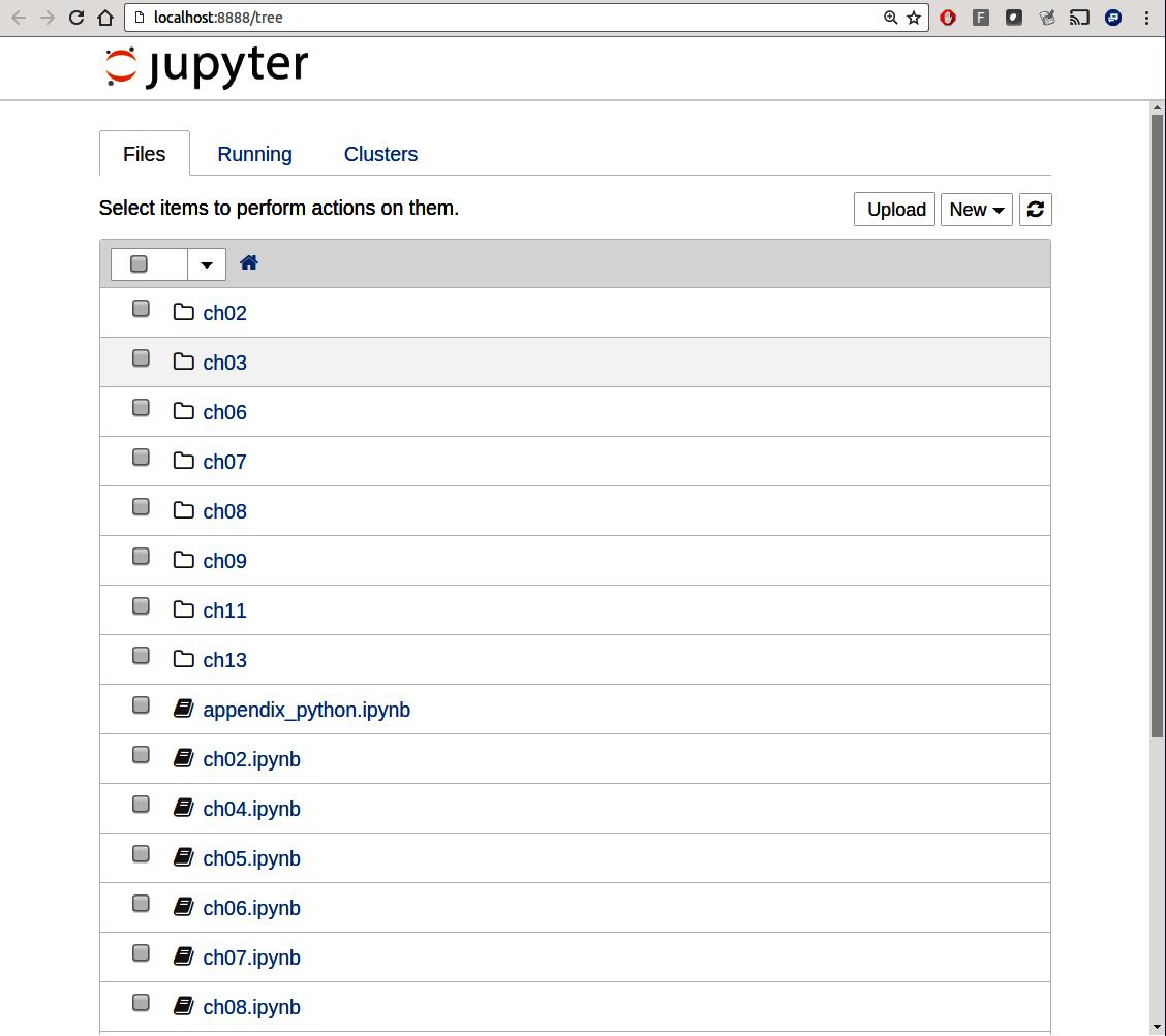
or http://127.0.0.1:8888/?token=0a77b52fefe52ab83e3c35dff8de121e4...On many platforms, Jupyter will automatically open in your default web browser (unless you start it with --no-browser). Otherwise, you can navigate to the HTTP address printed when you started the notebook, here http://localhost:8888/?token=0a77b52fefe52ab83e3c35dff8de121e4bb443a63f2d3055. See Figure 2.1 for what this looks like in Google Chrome.
Many people use Jupyter as a local computing environment, but it can also be deployed on servers and accessed remotely. I won't cover those details here, but I encourage you to explore this topic on the internet if it's relevant to your needs.
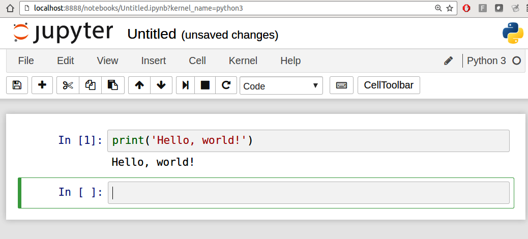
To create a new notebook, click the New button and select the "Python 3" option. You should see something like Figure 2.2. If this is your first time, try clicking on the empty code "cell" and entering a line of Python code. Then press Shift-Enter to execute it.
When you save the notebook (see "Save and Checkpoint" under the notebook File menu), it creates a file with the extension .ipynb. This is a self-contained file format that contains all of the content (including any evaluated code output) currently in the notebook. These can be loaded and edited by other Jupyter users.
To rename an open notebook, click on the notebook title at the top of the page and type the new title, pressing Enter when you are finished.
To load an existing notebook, put the file in the same directory where you started the notebook process (or in a subfolder within it), then click the name from the landing page. You can try it out with the notebooks from my wesm/pydata-book repository on GitHub. See Figure 2.3.
When you want to close a notebook, click the File menu and select "Close and Halt." If you simply close the browser tab, the Python process associated with the notebook will keep running in the background.
While the Jupyter notebook may feel like a distinct experience from the IPython shell, nearly all of the commands and tools in this chapter can be used in either environment.

Tab Completion
On the surface, the IPython shell looks like a cosmetically different version of the standard terminal Python interpreter (invoked with python). One of the major improvements over the standard Python shell is tab completion, found in many IDEs or other interactive computing analysis environments. While entering expressions in the shell, pressing the Tab key will search the namespace for any variables (objects, functions, etc.) matching the characters you have typed so far and show the results in a convenient drop-down menu:
In [1]: an_apple = 27

In [2]: an_example = 42

In [3]: an<Tab>
an_apple   an_example  any
In this example, note that IPython displayed both of the two variables I defined, as well as the built-in function any. Also, you can also complete methods and attributes on any object after typing a period:
In [3]: b = [1, 2, 3]

In [4]: b.<Tab>
append()  count()   insert()  reverse()
clear()   extend()  pop()     sort()
copy()    index()   remove()
The same is true for modules:
In [1]: import datetime

In [2]: datetime.<Tab>
date          MAXYEAR       timedelta
datetime      MINYEAR       timezone
datetime_CAPI time          tzinfo
Note that IPython by default hides methods and attributes starting with underscores, such as magic methods and internal “private” methods and attributes, in order to avoid cluttering the display (and confusing novice users!). These, too, can be tab-completed, but you must first type an underscore to see them. If you prefer to always see such methods in tab completion, you can change this setting in the IPython configuration. See the IPython documentation to find out how to do this.
Tab completion works in many contexts outside of searching the interactive namespace and completing object or module attributes. When typing anything that looks like a file path (even in a Python string), pressing the Tab key will complete anything on your computer’s filesystem matching what you’ve typed.
Combined with the %run command (see Appendix B.2.1: The %run Command), this functionality can save you many keystrokes.
Another area where tab completion saves time is in the completion of function keyword arguments (including the = sign!). See Figure 2.4.
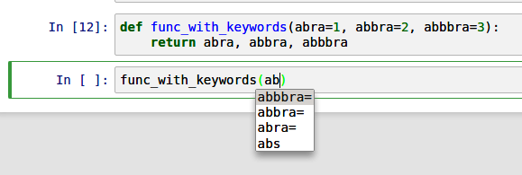
We'll have a closer look at functions in a little bit.
Introspection
Using a question mark (?) before or after a variable will display some general information about the object:
In [1]: b = [1, 2, 3]

In [2]: b?
Type:        list
String form: [1, 2, 3]
Length:      3
Docstring:
Built-in mutable sequence.

If no argument is given, the constructor creates a new empty list.
The argument must be an iterable if specified.

In [3]: print?
Docstring:
print(value, ..., sep=' ', end='\n', file=sys.stdout, flush=False)

Prints the values to a stream, or to sys.stdout by default.
Optional keyword arguments:
file:  a file-like object (stream); defaults to the current sys.stdout.
sep:   string inserted between values, default a space.
end:   string appended after the last value, default a newline.
flush: whether to forcibly flush the stream.
Type:      builtin_function_or_method
This is referred to as object introspection. If the object is a function or instance method, the docstring, if defined, will also be shown. Suppose we’d written the following function (which you can reproduce in IPython or Jupyter):
def add_numbers(a, b):
    """
    Add two numbers together

    Returns
    -------
    the_sum : type of arguments
    """
    return a + b
Then using ? shows us the docstring:
In [6]: add_numbers?
Signature: add_numbers(a, b)
Docstring:
Add two numbers together
Returns
-------
the_sum : type of arguments
File:      <ipython-input-9-6a548a216e27>
Type:      function
? has a final usage, which is for searching the IPython namespace in a manner similar to the standard Unix or Windows command line. A number of characters combined with the wildcard (*) will show all names matching the wildcard expression. For example, we could get a list of all functions in the top-level NumPy namespace containing load:
In [9]: import numpy as np

In [10]: np.*load*?
np.__loader__
np.load
np.loads
np.loadtxt
2.3 Python Language Basics
In this section, I will give you an overview of essential Python programming concepts and language mechanics. In the next chapter, I will go into more detail about Python data structures, functions, and other built-in tools.
Language Semantics
The Python language design is distinguished by its emphasis on readability, simplicity, and explicitness. Some people go so far as to liken it to “executable pseudocode.”
Indentation, not braces
Python uses whitespace (tabs or spaces) to structure code instead of using braces as in many other languages like R, C++, Java, and Perl. Consider a for loop from a sorting algorithm:
for x in array:
    if x < pivot:
        less.append(x)
    else:
        greater.append(x)
A colon denotes the start of an indented code block after which all of the code must be indented by the same amount until the end of the block.
Love it or hate it, significant whitespace is a fact of life for Python programmers. While it may seem foreign at first, you will hopefully grow accustomed to it in time.
I strongly recommend using four spaces as your default indentation and replacing tabs with four spaces. Many text editors have a setting that will replace tab stops with spaces automatically (do this!). IPython and Jupyter notebooks will automatically insert four spaces on new lines following a colon and replace tabs by four spaces.
As you can see by now, Python statements also do not need to be terminated by semicolons. Semicolons can be used, however, to separate multiple statements on a single line:
a = 5; b = 6; c = 7Putting multiple statements on one line is generally discouraged in Python as it can make code less readable.
Everything is an object
An important characteristic of the Python language is the consistency of its object model. Every number, string, data structure, function, class, module, and so on exists in the Python interpreter in its own “box,” which is referred to as a Python object. Each object has an associated type (e.g., integer, string, or function) and internal data. In practice this makes the language very flexible, as even functions can be treated like any other object.
Comments
Any text preceded by the hash mark (pound sign) # is ignored by the Python interpreter. This is often used to add comments to code. At times you may also want to exclude certain blocks of code without deleting them. One solution is to comment out the code:
results = []
for line in file_handle:
    # keep the empty lines for now
    # if len(line) == 0:
    #   continue
    results.append(line.replace("foo", "bar"))
Comments can also occur after a line of executed code. While some programmers prefer comments to be placed in the line preceding a particular line of code, this can be useful at times:
print("Reached this line") # Simple status reportFunction and object method calls
You call functions using parentheses and passing zero or more arguments, optionally assigning the returned value to a variable:
result = f(x, y, z)
g()
Almost every object in Python has attached functions, known as methods, that have access to the object’s internal contents. You can call them using the following syntax:
obj.some_method(x, y, z)Functions can take both positional and keyword arguments:
result = f(a, b, c, d=5, e="foo")We will look at this in more detail later.
Variables and argument passing
When assigning a variable (or name) in Python, you are creating a reference to the object shown on the righthand side of the equals sign. In practical terms, consider a list of integers:
In [8]: a = [1, 2, 3]Suppose we assign a to a new variable b:
In [9]: b = a

In [10]: b
Out[10]: [1, 2, 3]
In some languages, the assignment if b will cause the data [1, 2, 3] to be copied. In Python, a and b actually now refer to the same object, the original list [1, 2, 3] (see Figure 2.5 for a mock-up). You can prove this to yourself by appending an element to a and then examining b:
In [11]: a.append(4)

In [12]: b
Out[12]: [1, 2, 3, 4]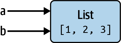
Understanding the semantics of references in Python, and when, how, and why data is copied, is especially critical when you are working with larger datasets in Python.
Assignment is also referred to as binding, as we are binding a name to an object. Variable names that have been assigned may occasionally be referred to as bound variables.
When you pass objects as arguments to a function, new local variables are created referencing the original objects without any copying. If you bind a new object to a variable inside a function, that will not overwrite a variable of the same name in the "scope" outside of the function (the "parent scope"). It is therefore possible to alter the internals of a mutable argument. Suppose we had the following function:
In [13]: def append_element(some_list, element):
   ....:     some_list.append(element)
Then we have:
In [14]: data = [1, 2, 3]

In [15]: append_element(data, 4)

In [16]: data
Out[16]: [1, 2, 3, 4]
Dynamic references, strong types
Variables in Python have no inherent type associated with them; a variable can refer to a different type of object simply by doing an assignment. There is no problem with the following:
In [17]: a = 5

In [18]: type(a)
Out[18]: int

In [19]: a = "foo"

In [20]: type(a)
Out[20]: str
Variables are names for objects within a particular namespace; the type information is stored in the object itself. Some observers might hastily conclude that Python is not a “typed language.” This is not true; consider this example:
In [21]: "5" + 5
---------------------------------------------------------------------------
TypeError                                 Traceback (most recent call last)
<ipython-input-21-7fe5aa79f268> in <module>
----> 1 "5" + 5
TypeError: can only concatenate str (not "int") to str
In some languages, the string '5' might get implicitly converted (or cast) to an integer, thus yielding 10. In other languages the integer 5 might be cast to a string, yielding the concatenated string '55'. In Python, such implicit casts are not allowed. In this regard we say that Python is a strongly typed language, which means that every object has a specific type (or class), and implicit conversions will occur only in certain permitted circumstances, such as:
In [22]: a = 4.5

In [23]: b = 2

# String formatting, to be visited later
In [24]: print(f"a is {type(a)}, b is {type(b)}")
a is <class 'float'>, b is <class 'int'>

In [25]: a / b
Out[25]: 2.25
Here, even though b is an integer, it is implicitly converted to a float for the division operation.
Knowing the type of an object is important, and it’s useful to be able to write functions that can handle many different kinds of input. You can check that an object is an instance of a particular type using the isinstance function:
In [26]: a = 5

In [27]: isinstance(a, int)
Out[27]: True
isinstance can accept a tuple of types if you want to check that an object’s type is among those present in the tuple:
In [28]: a = 5; b = 4.5

In [29]: isinstance(a, (int, float))
Out[29]: True

In [30]: isinstance(b, (int, float))
Out[30]: True
Attributes and methods
Objects in Python typically have both attributes (other Python objects stored “inside” the object) and methods (functions associated with an object that can have access to the object’s internal data). Both of them are accessed via the syntax <obj.attribute_name>:
In [1]: a = "foo"

In [2]: a.<Press Tab>
capitalize() index()        isspace()      removesuffix()  startswith()
casefold()   isprintable()  istitle()      replace()       strip()
center()     isalnum()      isupper()      rfind()         swapcase()
count()      isalpha()      join()         rindex()        title()
encode()     isascii()      ljust()        rjust()         translate()
endswith()   isdecimal()    lower()        rpartition()
expandtabs() isdigit()      lstrip()       rsplit()
find()       isidentifier() maketrans()    rstrip()
format()     islower()      partition()    split()
format_map() isnumeric()    removeprefix() splitlines()
Attributes and methods can also be accessed by name via the getattr function:
In [32]: getattr(a, "split")
Out[32]: <function str.split(sep=None, maxsplit=-1)>
While we will not extensively use the functions getattr and related functions hasattr and setattr in this book, they can be used very effectively to write generic, reusable code.
Duck typing
Often you may not care about the type of an object but rather only whether it has certain methods or behavior. This is sometimes called duck typing, after the saying "If it walks like a duck and quacks like a duck, then it's a duck." For example, you can verify that an object is iterable if it implements the iterator protocol. For many objects, this means it has an __iter__ “magic method,” though an alternative and better way to check is to try using the iter function:
In [33]: def isiterable(obj):
   ....:     try:
   ....:         iter(obj)
   ....:         return True
   ....:     except TypeError: # not iterable
   ....:         return False
This function would return True for strings as well as most Python collection types:
In [34]: isiterable("a string")
Out[34]: True

In [35]: isiterable([1, 2, 3])
Out[35]: True

In [36]: isiterable(5)
Out[36]: False
Imports
In Python, a module is simply a file with the .py extension containing Python code. Suppose we had the following module:
# some_module.py
PI = 3.14159

def f(x):
    return x + 2

def g(a, b):
    return a + b
If we wanted to access the variables and functions defined in some_module.py, from another file in the same directory we could do:
import some_module
result = some_module.f(5)
pi = some_module.PI
Or alternately:
from some_module import g, PI
result = g(5, PI)
By using the as keyword, you can give imports different variable names:
import some_module as sm
from some_module import PI as pi, g as gf

r1 = sm.f(pi)
r2 = gf(6, pi)
Binary operators and comparisons
Most of the binary math operations and comparisons use familiar mathematical syntax used in other programming languages:
In [37]: 5 - 7
Out[37]: -2

In [38]: 12 + 21.5
Out[38]: 33.5

In [39]: 5 <= 2
Out[39]: False
See Table 2.1 for all of the available binary operators.
| Operation | Description |
|---|---|
a + b |
Add a and b |
a - b |
Subtract b from a |
a * b |
Multiply a by b |
a / b |
Divide a by b |
a // b |
Floor-divide a by b, dropping any fractional remainder |
a ** b |
Raise a to the b power |
a & b |
True if both a and b are True; for integers, take the bitwise AND |
a | b |
True if either a or b is True; for integers, take the bitwise OR |
a ^ b |
For Booleans, True if a or b is True, but not both; for integers, take the bitwise EXCLUSIVE-OR |
a == b |
True if a equals b |
a != b |
True if a is not equal to b |
a < b, a <= b |
True if a is less than (less than or equal to) b |
a > b, a >= b |
True if a is greater than (greater than or equal to) b |
a is b |
True if a and b reference the same Python object |
a is not b |
True if a and b reference different Python objects |
To check if two variables refer to the same object, use the is keyword. Use is not to check that two objects are not the same:
In [40]: a = [1, 2, 3]

In [41]: b = a

In [42]: c = list(a)

In [43]: a is b
Out[43]: True

In [44]: a is not c
Out[44]: True
Since the list function always creates a new Python list (i.e., a copy), we can be sure that c is distinct from a. Comparing with is is not the same as the == operator, because in this case we have:
In [45]: a == c
Out[45]: True
A common use of is and is not is to check if a variable is None, since there is only one instance of None:
In [46]: a = None

In [47]: a is None
Out[47]: True
Mutable and immutable objects
Many objects in Python, such as lists, dictionaries, NumPy arrays, and most user-defined types (classes), are mutable. This means that the object or values that they contain can be modified:
In [48]: a_list = ["foo", 2, [4, 5]]

In [49]: a_list[2] = (3, 4)

In [50]: a_list
Out[50]: ['foo', 2, (3, 4)]
Others, like strings and tuples, are immutable, which means their internal data cannot be changed:
In [51]: a_tuple = (3, 5, (4, 5))

In [52]: a_tuple[1] = "four"
---------------------------------------------------------------------------
TypeError                                 Traceback (most recent call last)
<ipython-input-52-cd2a018a7529> in <module>
----> 1 a_tuple[1] = "four"
TypeError: 'tuple' object does not support item assignment
Remember that just because you can mutate an object does not mean that you always should. Such actions are known as side effects. For example, when writing a function, any side effects should be explicitly communicated to the user in the function’s documentation or comments. If possible, I recommend trying to avoid side effects and favor immutability, even though there may be mutable objects involved.
Scalar Types
Python has a small set of built-in types for handling numerical data, strings, Boolean (True or False) values, and dates and time. These "single value" types are sometimes called scalar types, and we refer to them in this book as scalars . See Table 2.2 for a list of the main scalar types. Date and time handling will be discussed separately, as these are provided by the datetime module in the standard library.
| Type | Description |
|---|---|
None |
The Python “null” value (only one instance of the None object exists) |
str |
String type; holds Unicode strings |
bytes |
Raw binary data |
float |
Double-precision floating-point number (note there is no separate double type) |
bool |
A Boolean True or False value |
int |
Arbitrary precision integer |
Numeric types
The primary Python types for numbers are int and float. An int can store arbitrarily large numbers:
In [53]: ival = 17239871

In [54]: ival ** 6
Out[54]: 26254519291092456596965462913230729701102721
Floating-point numbers are represented with the Python float type. Under the hood, each one is a double-precision value. They can also be expressed with scientific notation:
In [55]: fval = 7.243

In [56]: fval2 = 6.78e-5
Integer division not resulting in a whole number will always yield a floating-point number:
In [57]: 3 / 2
Out[57]: 1.5
To get C-style integer division (which drops the fractional part if the result is not a whole number), use the floor division operator //:
In [58]: 3 // 2
Out[58]: 1
Strings
Many people use Python for its built-in string handling capabilities. You can write string literals using either single quotes ' or double quotes " (double quotes are generally favored):
a = 'one way of writing a string'
b = "another way"
The Python string type is str.
For multiline strings with line breaks, you can use triple quotes, either ''' or """:
c = """
This is a longer string that
spans multiple lines
"""
It may surprise you that this string c actually contains four lines of text; the line breaks after """ and after lines are included in the string. We can count the new line characters with the count method on c:
In [60]: c.count("\n")
Out[60]: 3
Python strings are immutable; you cannot modify a string:
In [61]: a = "this is a string"

In [62]: a[10] = "f"
---------------------------------------------------------------------------
TypeError                                 Traceback (most recent call last)
<ipython-input-62-3b2d95f10db4> in <module>
----> 1 a[10] = "f"
TypeError: 'str' object does not support item assignment
To interpret this error message, read from the bottom up. We tried to replace the character (the "item") at position 10 with the letter "f", but this is not allowed for string objects. If we need to modify a string, we have to use a function or method that creates a new string, such as the string replace method:
In [63]: b = a.replace("string", "longer string")

In [64]: b
Out[64]: 'this is a longer string'
Afer this operation, the variable a is unmodified:
In [65]: a
Out[65]: 'this is a string'
Many Python objects can be converted to a string using the str function:
In [66]: a = 5.6

In [67]: s = str(a)

In [68]: print(s)
5.6
Strings are a sequence of Unicode characters and therefore can be treated like other sequences, such as lists and tuples:
In [69]: s = "python"

In [70]: list(s)
Out[70]: ['p', 'y', 't', 'h', 'o', 'n']

In [71]: s[:3]
Out[71]: 'pyt'
The syntax s[:3] is called slicing and is implemented for many kinds of Python sequences. This will be explained in more detail later on, as it is used extensively in this book.
The backslash character \ is an escape character, meaning that it is used to specify special characters like newline \n or Unicode characters. To write a string literal with backslashes, you need to escape them:
In [72]: s = "12\\34"

In [73]: print(s)
12\34
If you have a string with a lot of backslashes and no special characters, you might find this a bit annoying. Fortunately you can preface the leading quote of the string with r, which means that the characters should be interpreted as is:
In [74]: s = r"this\has\no\special\characters"

In [75]: s
Out[75]: 'this\\has\\no\\special\\characters'
The r stands for raw.
Adding two strings together concatenates them and produces a new string:
In [76]: a = "this is the first half "

In [77]: b = "and this is the second half"

In [78]: a + b
Out[78]: 'this is the first half and this is the second half'
String templating or formatting is another important topic. The number of ways to do so has expanded with the advent of Python 3, and here I will briefly describe the mechanics of one of the main interfaces. String objects have a format method that can be used to substitute formatted arguments into the string, producing a new string:
In [79]: template = "{0:.2f} {1:s} are worth US${2:d}"In this string:
{0:.2f}means to format the first argument as a floating-point number with two decimal places.{1:s}means to format the second argument as a string.{2:d}means to format the third argument as an exact integer.
To substitute arguments for these format parameters, we pass a sequence of arguments to the format method:
In [80]: template.format(88.46, "Argentine Pesos", 1)
Out[80]: '88.46 Argentine Pesos are worth US$1'
Python 3.6 introduced a new feature called f-strings (short for formatted string literals) which can make creating formatted strings even more convenient. To create an f-string, write the character f immediately preceding a string literal. Within the string, enclose Python expressions in curly braces to substitute the value of the expression into the formatted string:
In [81]: amount = 10

In [82]: rate = 88.46

In [83]: currency = "Pesos"

In [84]: result = f"{amount} {currency} is worth US${amount / rate}"
Format specifiers can be added after each expression using the same syntax as with the string templates above:
In [85]: f"{amount} {currency} is worth US${amount / rate:.2f}"
Out[85]: '10 Pesos is worth US$0.11'
String formatting is a deep topic; there are multiple methods and numerous options and tweaks available to control how values are formatted in the resulting string. To learn more, consult the official Python documentation.
Bytes and Unicode
In modern Python (i.e., Python 3.0 and up), Unicode has become the first-class string type to enable more consistent handling of ASCII and non-ASCII text. In older versions of Python, strings were all bytes without any explicit Unicode encoding. You could convert to Unicode assuming you knew the character encoding. Here is an example Unicode string with non-ASCII characters:
In [86]: val = "español"

In [87]: val
Out[87]: 'español'
We can convert this Unicode string to its UTF-8 bytes representation using the encode method:
In [88]: val_utf8 = val.encode("utf-8")

In [89]: val_utf8
Out[89]: b'espa\xc3\xb1ol'

In [90]: type(val_utf8)
Out[90]: bytes
Assuming you know the Unicode encoding of a bytes object, you can go back using the decode method:
In [91]: val_utf8.decode("utf-8")
Out[91]: 'español'
While it is now preferable to use UTF-8 for any encoding, for historical reasons you may encounter data in any number of different encodings:
In [92]: val.encode("latin1")
Out[92]: b'espa\xf1ol'

In [93]: val.encode("utf-16")
Out[93]: b'\xff\xfee\x00s\x00p\x00a\x00\xf1\x00o\x00l\x00'

In [94]: val.encode("utf-16le")
Out[94]: b'e\x00s\x00p\x00a\x00\xf1\x00o\x00l\x00'
It is most common to encounter bytes objects in the context of working with files, where implicitly decoding all data to Unicode strings may not be desired.
Booleans
The two Boolean values in Python are written as True and False. Comparisons and other conditional expressions evaluate to either True or False. Boolean values are combined with the and and or keywords:
In [95]: True and True
Out[95]: True

In [96]: False or True
Out[96]: True
When converted to numbers, False becomes 0 and True becomes 1:
In [97]: int(False)
Out[97]: 0

In [98]: int(True)
Out[98]: 1
The keyword not flips a Boolean value from True to False or vice versa:
In [99]: a = True

In [100]: b = False

In [101]: not a
Out[101]: False

In [102]: not b
Out[102]: True
Type casting
The str, bool, int, and float types are also functions that can be used to cast values to those types:
In [103]: s = "3.14159"

In [104]: fval = float(s)

In [105]: type(fval)
Out[105]: float

In [106]: int(fval)
Out[106]: 3

In [107]: bool(fval)
Out[107]: True

In [108]: bool(0)
Out[108]: False
Note that most nonzero values when cast to bool become True.
None
None is the Python null value type:
In [109]: a = None

In [110]: a is None
Out[110]: True

In [111]: b = 5

In [112]: b is not None
Out[112]: True
None is also a common default value for function arguments:
def add_and_maybe_multiply(a, b, c=None):
    result = a + b

    if c is not None:
        result = result * c

    return result
Dates and times
The built-in Python datetime module provides datetime, date, and time types. The datetime type combines the information stored in date and time and is the most commonly used:
In [113]: from datetime import datetime, date, time

In [114]: dt = datetime(2011, 10, 29, 20, 30, 21)

In [115]: dt.day
Out[115]: 29

In [116]: dt.minute
Out[116]: 30
Given a datetime instance, you can extract the equivalent date and time objects by calling methods on the datetime of the same name:
In [117]: dt.date()
Out[117]: datetime.date(2011, 10, 29)

In [118]: dt.time()
Out[118]: datetime.time(20, 30, 21)
The strftime method formats a datetime as a string:
In [119]: dt.strftime("%Y-%m-%d %H:%M")
Out[119]: '2011-10-29 20:30'
Strings can be converted (parsed) into datetime objects with the strptime function:
In [120]: datetime.strptime("20091031", "%Y%m%d")
Out[120]: datetime.datetime(2009, 10, 31, 0, 0)
See Table 11.2 for a full list of format specifications.
When you are aggregating or otherwise grouping time series data, it will occasionally be useful to replace time fields of a series of datetimes—for example, replacing the minute and second fields with zero:
In [121]: dt_hour = dt.replace(minute=0, second=0)

In [122]: dt_hour
Out[122]: datetime.datetime(2011, 10, 29, 20, 0)
Since datetime.datetime is an immutable type, methods like these always produce new objects. So in the previous example, dt is not modified by replace:
In [123]: dt
Out[123]: datetime.datetime(2011, 10, 29, 20, 30, 21)
The difference of two datetime objects produces a datetime.timedelta type:
In [124]: dt2 = datetime(2011, 11, 15, 22, 30)

In [125]: delta = dt2 - dt

In [126]: delta
Out[126]: datetime.timedelta(days=17, seconds=7179)

In [127]: type(delta)
Out[127]: datetime.timedelta
The output timedelta(17, 7179) indicates that the timedelta encodes an offset of 17 days and 7,179 seconds.
Adding a timedelta to a datetime produces a new shifted datetime:
In [128]: dt
Out[128]: datetime.datetime(2011, 10, 29, 20, 30, 21)

In [129]: dt + delta
Out[129]: datetime.datetime(2011, 11, 15, 22, 30)
Control Flow
Python has several built-in keywords for conditional logic, loops, and other standard control flow concepts found in other programming languages.
if, elif, and else
The if statement is one of the most well-known control flow statement types. It checks a condition that, if True, evaluates the code in the block that follows:
x = -5
if x < 0:
    print("It's negative")
An if statement can be optionally followed by one or more elif blocks and a catchall else block if all of the conditions are False:
if x < 0:
    print("It's negative")
elif x == 0:
    print("Equal to zero")
elif 0 < x < 5:
    print("Positive but smaller than 5")
else:
    print("Positive and larger than or equal to 5")
If any of the conditions are True, no further elif or else blocks will be reached. With a compound condition using and or or, conditions are evaluated left to right and will short-circuit:
In [130]: a = 5; b = 7

In [131]: c = 8; d = 4

In [132]: if a < b or c > d:
   .....:     print("Made it")
Made it
In this example, the comparison c > d never gets evaluated because the first comparison was True.
It is also possible to chain comparisons:
In [133]: 4 > 3 > 2 > 1
Out[133]: True
for loops
for loops are for iterating over a collection (like a list or tuple) or an iterater. The standard syntax for a for loop is:
for value in collection:
    # do something with value
You can advance a for loop to the next iteration, skipping the remainder of the block, using the continue keyword. Consider this code, which sums up integers in a list and skips None values:
sequence = [1, 2, None, 4, None, 5]
total = 0
for value in sequence:
    if value is None:
        continue
    total += value
A for loop can be exited altogether with the break keyword. This code sums elements of the list until a 5 is reached:
sequence = [1, 2, 0, 4, 6, 5, 2, 1]
total_until_5 = 0
for value in sequence:
    if value == 5:
        break
    total_until_5 += value
The break keyword only terminates the innermost for loop; any outer for loops will continue to run:
In [134]: for i in range(4):
   .....:     for j in range(4):
   .....:         if j > i:
   .....:             break
   .....:         print((i, j))
   .....:
(0, 0)
(1, 0)
(1, 1)
(2, 0)
(2, 1)
(2, 2)
(3, 0)
(3, 1)
(3, 2)
(3, 3)
As we will see in more detail, if the elements in the collection or iterator are sequences (tuples or lists, say), they can be conveniently unpacked into variables in the for loop statement:
for a, b, c in iterator:
    # do something
while loops
A while loop specifies a condition and a block of code that is to be executed until the condition evaluates to False or the loop is explicitly ended with break:
x = 256
total = 0
while x > 0:
    if total > 500:
        break
    total += x
    x = x // 2
pass
pass is the “no-op” (or "do nothing") statement in Python. It can be used in blocks where no action is to be taken (or as a placeholder for code not yet implemented); it is required only because Python uses whitespace to delimit blocks:
if x < 0:
    print("negative!")
elif x == 0:
    # TODO: put something smart here
    pass
else:
    print("positive!")
range
The range function generates a sequence of evenly spaced integers:
In [135]: range(10)
Out[135]: range(0, 10)

In [136]: list(range(10))
Out[136]: [0, 1, 2, 3, 4, 5, 6, 7, 8, 9]
A start, end, and step (which may be negative) can be given:
In [137]: list(range(0, 20, 2))
Out[137]: [0, 2, 4, 6, 8, 10, 12, 14, 16, 18]

In [138]: list(range(5, 0, -1))
Out[138]: [5, 4, 3, 2, 1]
As you can see, range produces integers up to but not including the endpoint. A common use of range is for iterating through sequences by index:
In [139]: seq = [1, 2, 3, 4]

In [140]: for i in range(len(seq)):
   .....:     print(f"element {i}: {seq[i]}")
element 0: 1
element 1: 2
element 2: 3
element 3: 4
While you can use functions like list to store all the integers generated by range in some other data structure, often the default iterator form will be what you want. This snippet sums all numbers from 0 to 99,999 that are multiples of 3 or 5:
In [141]: total = 0

In [142]: for i in range(100_000):
   .....:     # % is the modulo operator
   .....:     if i % 3 == 0 or i % 5 == 0:
   .....:         total += i

In [143]: print(total)
2333316668
While the range generated can be arbitrarily large, the memory use at any given time may be very small.
2.4 Conclusion
This chapter provided a brief introduction to some basic Python language concepts and the IPython and Jupyter programming environments. In the next chapter, I will discuss many built-in data types, functions, and input-output utilities that will be used continuously throughout the rest of the book.