11 Time Series
Time series data is an important form of structured data in many different fields, such as finance, economics, ecology, neuroscience, and physics. Anything that is recorded repeatedly at many points in time forms a time series. Many time series are fixed frequency, which is to say that data points occur at regular intervals according to some rule, such as every 15 seconds, every 5 minutes, or once per month. Time series can also be irregular without a fixed unit of time or offset between units. How you mark and refer to time series data depends on the application, and you may have one of the following:
- Timestamps
-
Specific instants in time.
- Fixed periods
-
Such as the whole month of January 2017, or the whole year 2020.
- Intervals of time
-
Indicated by a start and end timestamp. Periods can be thought of as special cases of intervals.
- Experiment or elapsed time
-
Each timestamp is a measure of time relative to a particular start time (e.g., the diameter of a cookie baking each second since being placed in the oven), starting from 0.
In this chapter, I am mainly concerned with time series in the first three categories, though many of the techniques can be applied to experimental time series where the index may be an integer or floating-point number indicating elapsed time from the start of the experiment. The simplest kind of time series is indexed by timestamp.
pandas also supports indexes based on timedeltas, which can be a useful way of representing experiment or elapsed time. We do not explore timedelta indexes in this book, but you can learn more in the pandas documentation.
pandas provides many built-in time series tools and algorithms. You can efficiently work with large time series, and slice and dice, aggregate, and resample irregular- and fixed-frequency time series. Some of these tools are useful for financial and economics applications, but you could certainly use them to analyze server log data, too.
As with the rest of the chapters, we start by importing NumPy and pandas:
In [12]: import numpy as np

In [13]: import pandas as pd
11.1 Date and Time Data Types and Tools
The Python standard library includes data types for date and time data, as well as calendar-related functionality. The datetime, time, and calendar modules are the main places to start. The datetime.datetime type, or simply datetime, is widely used:
In [14]: from datetime import datetime

In [15]: now = datetime.now()

In [16]: now
Out[16]: datetime.datetime(2023, 4, 12, 13, 9, 16, 484533)

In [17]: now.year, now.month, now.day
Out[17]: (2023, 4, 12)
datetime stores both the date and time down to the microsecond. datetime.timedelta, or simply timedelta, represents the temporal difference between two datetime objects:
In [18]: delta = datetime(2011, 1, 7) - datetime(2008, 6, 24, 8, 15)

In [19]: delta
Out[19]: datetime.timedelta(days=926, seconds=56700)

In [20]: delta.days
Out[20]: 926

In [21]: delta.seconds
Out[21]: 56700
You can add (or subtract) a timedelta or multiple thereof to a datetime object to yield a new shifted object:
In [22]: from datetime import timedelta

In [23]: start = datetime(2011, 1, 7)

In [24]: start + timedelta(12)
Out[24]: datetime.datetime(2011, 1, 19, 0, 0)

In [25]: start - 2 * timedelta(12)
Out[25]: datetime.datetime(2010, 12, 14, 0, 0)
Table 11.1 summarizes the data types in the datetime module. While this chapter is mainly concerned with the data types in pandas and higher-level time series manipulation, you may encounter the datetime-based types in many other places in Python in the wild.
| Type | Description |
|---|---|
date |
Store calendar date (year, month, day) using the Gregorian calendar |
time |
Store time of day as hours, minutes, seconds, and microseconds |
datetime |
Store both date and time |
timedelta |
The difference between two datetime values (as days, seconds, and microseconds) |
tzinfo |
Base type for storing time zone information |
Converting Between String and Datetime
You can format datetime objects and pandas Timestamp objects, which I’ll introduce later, as strings using str or the strftime method, passing a format specification:
In [26]: stamp = datetime(2011, 1, 3)

In [27]: str(stamp)
Out[27]: '2011-01-03 00:00:00'

In [28]: stamp.strftime("%Y-%m-%d")
Out[28]: '2011-01-03'
See Table 11.2 for a complete list of the format codes.
| Type | Description |
|---|---|
%Y |
Four-digit year |
%y |
Two-digit year |
%m |
Two-digit month [01, 12] |
%d |
Two-digit day [01, 31] |
%H |
Hour (24-hour clock) [00, 23] |
%I |
Hour (12-hour clock) [01, 12] |
%M |
Two-digit minute [00, 59] |
%S |
Second [00, 61] (seconds 60, 61 account for leap seconds) |
%f |
Microsecond as an integer, zero-padded (from 000000 to 999999) |
%j |
Day of the year as a zero-padded integer (from 001 to 336) |
%w |
Weekday as an integer [0 (Sunday), 6] |
%u |
Weekday as an integer starting from 1, where 1 is Monday. |
%U |
Week number of the year [00, 53]; Sunday is considered the first day of the week, and days before the first Sunday of the year are “week 0” |
%W |
Week number of the year [00, 53]; Monday is considered the first day of the week, and days before the first Monday of the year are “week 0” |
%z |
UTC time zone offset as +HHMM or -HHMM; empty if time zone naive |
%Z |
Time zone name as a string, or empty string if no time zone |
%F |
Shortcut for %Y-%m-%d (e.g., 2012-4-18) |
%D |
Shortcut for %m/%d/%y (e.g., 04/18/12) |
You can use many of the same format codes to convert strings to dates using datetime.strptime (but some codes, like %F, cannot be used):
In [29]: value = "2011-01-03"

In [30]: datetime.strptime(value, "%Y-%m-%d")
Out[30]: datetime.datetime(2011, 1, 3, 0, 0)

In [31]: datestrs = ["7/6/2011", "8/6/2011"]

In [32]: [datetime.strptime(x, "%m/%d/%Y") for x in datestrs]
Out[32]:
[datetime.datetime(2011, 7, 6, 0, 0),
 datetime.datetime(2011, 8, 6, 0, 0)]
datetime.strptime is one way to parse a date with a known format.
pandas is generally oriented toward working with arrays of dates, whether used as an axis index or a column in a DataFrame. The pandas.to_datetime method parses many different kinds of date representations. Standard date formats like ISO 8601 can be parsed quickly:
In [33]: datestrs = ["2011-07-06 12:00:00", "2011-08-06 00:00:00"]

In [34]: pd.to_datetime(datestrs)
Out[34]: DatetimeIndex(['2011-07-06 12:00:00', '2011-08-06 00:00:00'], dtype='dat
etime64[ns]', freq=None)
It also handles values that should be considered missing (None, empty string, etc.):
In [35]: idx = pd.to_datetime(datestrs + [None])

In [36]: idx
Out[36]: DatetimeIndex(['2011-07-06 12:00:00', '2011-08-06 00:00:00', 'NaT'], dty
pe='datetime64[ns]', freq=None)

In [37]: idx[2]
Out[37]: NaT

In [38]: pd.isna(idx)
Out[38]: array([False, False,  True])
NaT (Not a Time) is pandas’s null value for timestamp data.
dateutil.parser is a useful but imperfect tool. Notably, it will recognize some strings as dates that you might prefer that it didn’t; for example, "42" will be parsed as the year 2042 with today’s calendar date.
datetime objects also have a number of locale-specific formatting options for systems in other countries or languages. For example, the abbreviated month names will be different on German or French systems compared with English systems. See Table 11.3 for a listing.
| Type | Description |
|---|---|
%a |
Abbreviated weekday name |
%A |
Full weekday name |
%b |
Abbreviated month name |
%B |
Full month name |
%c |
Full date and time (e.g., ‘Tue 01 May 2012 04:20:57 PM’) |
%p |
Locale equivalent of AM or PM |
%x |
Locale-appropriate formatted date (e.g., in the United States, May 1, 2012 yields ‘05/01/2012’) |
%X |
Locale-appropriate time (e.g., ‘04:24:12 PM’) |
11.2 Time Series Basics
A basic kind of time series object in pandas is a Series indexed by timestamps, which is often represented outside of pandas as Python strings or datetime objects:
In [39]: dates = [datetime(2011, 1, 2), datetime(2011, 1, 5),
   ....:          datetime(2011, 1, 7), datetime(2011, 1, 8),
   ....:          datetime(2011, 1, 10), datetime(2011, 1, 12)]

In [40]: ts = pd.Series(np.random.standard_normal(6), index=dates)

In [41]: ts
Out[41]:
2011-01-02   -0.204708
2011-01-05    0.478943
2011-01-07   -0.519439
2011-01-08   -0.555730
2011-01-10    1.965781
2011-01-12    1.393406
dtype: float64
Under the hood, these datetime objects have been put in a DatetimeIndex:
In [42]: ts.index
Out[42]:
DatetimeIndex(['2011-01-02', '2011-01-05', '2011-01-07', '2011-01-08',
               '2011-01-10', '2011-01-12'],
              dtype='datetime64[ns]', freq=None)
Like other Series, arithmetic operations between differently indexed time series automatically align on the dates:
In [43]: ts + ts[::2]
Out[43]:
2011-01-02   -0.409415
2011-01-05         NaN
2011-01-07   -1.038877
2011-01-08         NaN
2011-01-10    3.931561
2011-01-12         NaN
dtype: float64
Recall that ts[::2] selects every second element in ts.
pandas stores timestamps using NumPy’s datetime64 data type at the nanosecond resolution:
In [44]: ts.index.dtype
Out[44]: dtype('<M8[ns]')
Scalar values from a DatetimeIndex are pandas Timestamp objects:
In [45]: stamp = ts.index[0]

In [46]: stamp
Out[46]: Timestamp('2011-01-02 00:00:00')
A pandas.Timestamp can be substituted most places where you would use a datetime object. The reverse is not true, however, because pandas.Timestamp can store nanosecond precision data, while datetime stores only up to microseconds. Additionally, pandas.Timestamp can store frequency information (if any) and understands how to do time zone conversions and other kinds of manipulations. More on both of these things later in Time Zone Handling.
Indexing, Selection, Subsetting
Time series behaves like any other Series when you are indexing and selecting data based on the label:
In [47]: stamp = ts.index[2]

In [48]: ts[stamp]
Out[48]: -0.5194387150567381
As a convenience, you can also pass a string that is interpretable as a date:
In [49]: ts["2011-01-10"]
Out[49]: 1.9657805725027142
For longer time series, a year or only a year and month can be passed to easily select slices of data (pandas.date_range is discussed in more detail in Generating Date Ranges):
In [50]: longer_ts = pd.Series(np.random.standard_normal(1000),
   ....:                       index=pd.date_range("2000-01-01", periods=1000))

In [51]: longer_ts
Out[51]:
2000-01-01    0.092908
2000-01-02    0.281746
2000-01-03    0.769023
2000-01-04    1.246435
2000-01-05    1.007189
                ...
2002-09-22    0.930944
2002-09-23   -0.811676
2002-09-24   -1.830156
2002-09-25   -0.138730
2002-09-26    0.334088
Freq: D, Length: 1000, dtype: float64

In [52]: longer_ts["2001"]
Out[52]:
2001-01-01    1.599534
2001-01-02    0.474071
2001-01-03    0.151326
2001-01-04   -0.542173
2001-01-05   -0.475496
                ...
2001-12-27    0.057874
2001-12-28   -0.433739
2001-12-29    0.092698
2001-12-30   -1.397820
2001-12-31    1.457823
Freq: D, Length: 365, dtype: float64
Here, the string "2001" is interpreted as a year and selects that time period. This also works if you specify the month:
In [53]: longer_ts["2001-05"]
Out[53]:
2001-05-01   -0.622547
2001-05-02    0.936289
2001-05-03    0.750018
2001-05-04   -0.056715
2001-05-05    2.300675
                ...
2001-05-27    0.235477
2001-05-28    0.111835
2001-05-29   -1.251504
2001-05-30   -2.949343
2001-05-31    0.634634
Freq: D, Length: 31, dtype: float64
Slicing with datetime objects works as well:
In [54]: ts[datetime(2011, 1, 7):]
Out[54]:
2011-01-07   -0.519439
2011-01-08   -0.555730
2011-01-10    1.965781
2011-01-12    1.393406
dtype: float64

In [55]: ts[datetime(2011, 1, 7):datetime(2011, 1, 10)]
Out[55]:
2011-01-07   -0.519439
2011-01-08   -0.555730
2011-01-10    1.965781
dtype: float64
Because most time series data is ordered chronologically, you can slice with timestamps not contained in a time series to perform a range query:
In [56]: ts
Out[56]:
2011-01-02   -0.204708
2011-01-05    0.478943
2011-01-07   -0.519439
2011-01-08   -0.555730
2011-01-10    1.965781
2011-01-12    1.393406
dtype: float64

In [57]: ts["2011-01-06":"2011-01-11"]
Out[57]:
2011-01-07   -0.519439
2011-01-08   -0.555730
2011-01-10    1.965781
dtype: float64
As before, you can pass a string date, datetime, or timestamp. Remember that slicing in this manner produces views on the source time series, like slicing NumPy arrays. This means that no data is copied, and modifications on the slice will be reflected in the original data.
There is an equivalent instance method, truncate, that slices a Series between two dates:
In [58]: ts.truncate(after="2011-01-09")
Out[58]:
2011-01-02   -0.204708
2011-01-05    0.478943
2011-01-07   -0.519439
2011-01-08   -0.555730
dtype: float64
All of this holds true for DataFrame as well, indexing on its rows:
In [59]: dates = pd.date_range("2000-01-01", periods=100, freq="W-WED")

In [60]: long_df = pd.DataFrame(np.random.standard_normal((100, 4)),
   ....:                        index=dates,
   ....:                        columns=["Colorado", "Texas",
   ....:                                 "New York", "Ohio"])

In [61]: long_df.loc["2001-05"]
Out[61]:
            Colorado     Texas  New York      Ohio
2001-05-02 -0.006045  0.490094 -0.277186 -0.707213
2001-05-09 -0.560107  2.735527  0.927335  1.513906
2001-05-16  0.538600  1.273768  0.667876 -0.969206
2001-05-23  1.676091 -0.817649  0.050188  1.951312
2001-05-30  3.260383  0.963301  1.201206 -1.852001
Time Series with Duplicate Indices
In some applications, there may be multiple data observations falling on a particular timestamp. Here is an example:
In [62]: dates = pd.DatetimeIndex(["2000-01-01", "2000-01-02", "2000-01-02",
   ....:                           "2000-01-02", "2000-01-03"])

In [63]: dup_ts = pd.Series(np.arange(5), index=dates)

In [64]: dup_ts
Out[64]:
2000-01-01    0
2000-01-02    1
2000-01-02    2
2000-01-02    3
2000-01-03    4
dtype: int64
We can tell that the index is not unique by checking its is_unique property:
In [65]: dup_ts.index.is_unique
Out[65]: False
Indexing into this time series will now either produce scalar values or slices, depending on whether a timestamp is duplicated:
In [66]: dup_ts["2000-01-03"]  # not duplicated
Out[66]: 4

In [67]: dup_ts["2000-01-02"]  # duplicated
Out[67]:
2000-01-02    1
2000-01-02    2
2000-01-02    3
dtype: int64
Suppose you wanted to aggregate the data having nonunique timestamps. One way to do this is to use groupby and pass level=0 (the one and only level):
In [68]: grouped = dup_ts.groupby(level=0)

In [69]: grouped.mean()
Out[69]:
2000-01-01    0.0
2000-01-02    2.0
2000-01-03    4.0
dtype: float64

In [70]: grouped.count()
Out[70]:
2000-01-01    1
2000-01-02    3
2000-01-03    1
dtype: int64
11.3 Date Ranges, Frequencies, and Shifting
Generic time series in pandas are assumed to be irregular; that is, they have no fixed frequency. For many applications this is sufficient. However, it’s often desirable to work relative to a fixed frequency, such as daily, monthly, or every 15 minutes, even if that means introducing missing values into a time series. Fortunately, pandas has a full suite of standard time series frequencies and tools for resampling (discussed in more detail later in Resampling and Frequency Conversion), inferring frequencies, and generating fixed-frequency date ranges. For example, you can convert the sample time series to fixed daily frequency by calling resample:
In [71]: ts
Out[71]:
2011-01-02   -0.204708
2011-01-05    0.478943
2011-01-07   -0.519439
2011-01-08   -0.555730
2011-01-10    1.965781
2011-01-12    1.393406
dtype: float64

In [72]: resampler = ts.resample("D")

In [73]: resampler
Out[73]: <pandas.core.resample.DatetimeIndexResampler object at 0x17b0e7bb0>
The string "D" is interpreted as daily frequency.
Conversion between frequencies or resampling is a big enough topic to have its own section later (Resampling and Frequency Conversion). Here, I’ll show you how to use the base frequencies and multiples thereof.
Generating Date Ranges
While I used it previously without explanation, pandas.date_range is responsible for generating a DatetimeIndex with an indicated length according to a particular frequency:
In [74]: index = pd.date_range("2012-04-01", "2012-06-01")

In [75]: index
Out[75]:
DatetimeIndex(['2012-04-01', '2012-04-02', '2012-04-03', '2012-04-04',
               '2012-04-05', '2012-04-06', '2012-04-07', '2012-04-08',
               '2012-04-09', '2012-04-10', '2012-04-11', '2012-04-12',
               '2012-04-13', '2012-04-14', '2012-04-15', '2012-04-16',
               '2012-04-17', '2012-04-18', '2012-04-19', '2012-04-20',
               '2012-04-21', '2012-04-22', '2012-04-23', '2012-04-24',
               '2012-04-25', '2012-04-26', '2012-04-27', '2012-04-28',
               '2012-04-29', '2012-04-30', '2012-05-01', '2012-05-02',
               '2012-05-03', '2012-05-04', '2012-05-05', '2012-05-06',
               '2012-05-07', '2012-05-08', '2012-05-09', '2012-05-10',
               '2012-05-11', '2012-05-12', '2012-05-13', '2012-05-14',
               '2012-05-15', '2012-05-16', '2012-05-17', '2012-05-18',
               '2012-05-19', '2012-05-20', '2012-05-21', '2012-05-22',
               '2012-05-23', '2012-05-24', '2012-05-25', '2012-05-26',
               '2012-05-27', '2012-05-28', '2012-05-29', '2012-05-30',
               '2012-05-31', '2012-06-01'],
              dtype='datetime64[ns]', freq='D')
By default, pandas.date_range generates daily timestamps. If you pass only a start or end date, you must pass a number of periods to generate:
In [76]: pd.date_range(start="2012-04-01", periods=20)
Out[76]:
DatetimeIndex(['2012-04-01', '2012-04-02', '2012-04-03', '2012-04-04',
               '2012-04-05', '2012-04-06', '2012-04-07', '2012-04-08',
               '2012-04-09', '2012-04-10', '2012-04-11', '2012-04-12',
               '2012-04-13', '2012-04-14', '2012-04-15', '2012-04-16',
               '2012-04-17', '2012-04-18', '2012-04-19', '2012-04-20'],
              dtype='datetime64[ns]', freq='D')

In [77]: pd.date_range(end="2012-06-01", periods=20)
Out[77]:
DatetimeIndex(['2012-05-13', '2012-05-14', '2012-05-15', '2012-05-16',
               '2012-05-17', '2012-05-18', '2012-05-19', '2012-05-20',
               '2012-05-21', '2012-05-22', '2012-05-23', '2012-05-24',
               '2012-05-25', '2012-05-26', '2012-05-27', '2012-05-28',
               '2012-05-29', '2012-05-30', '2012-05-31', '2012-06-01'],
              dtype='datetime64[ns]', freq='D')
The start and end dates define strict boundaries for the generated date index. For example, if you wanted a date index containing the last business day of each month, you would pass the "BM" frequency (business end of month; see a more complete listing of frequencies in Table 11.4), and only dates falling on or inside the date interval will be included:
In [78]: pd.date_range("2000-01-01", "2000-12-01", freq="BM")
Out[78]:
DatetimeIndex(['2000-01-31', '2000-02-29', '2000-03-31', '2000-04-28',
               '2000-05-31', '2000-06-30', '2000-07-31', '2000-08-31',
               '2000-09-29', '2000-10-31', '2000-11-30'],
dtype='datetime64[ns]', freq='BM')| Alias | Offset type | Description |
|---|---|---|
D |
Day |
Calendar daily |
B |
BusinessDay |
Business daily |
H |
Hour |
Hourly |
T or min |
Minute |
Once a minute |
S |
Second |
Once a second |
L or ms |
Milli |
Millisecond (1/1,000 of 1 second) |
U |
Micro |
Microsecond (1/1,000,000 of 1 second) |
M |
MonthEnd |
Last calendar day of month |
BM |
BusinessMonthEnd |
Last business day (weekday) of month |
MS |
MonthBegin |
First calendar day of month |
BMS |
BusinessMonthBegin |
First weekday of month |
W-MON, W-TUE, ... |
Week |
Weekly on given day of week (MON, TUE, WED, THU, FRI, SAT, or SUN) |
WOM-1MON, WOM-2MON, ... |
WeekOfMonth |
Generate weekly dates in the first, second, third, or fourth week of the month (e.g., WOM-3FRI for the third Friday of each month) |
Q-JAN, Q-FEB, ... |
QuarterEnd |
Quarterly dates anchored on last calendar day of each month, for year ending in indicated month (JAN, FEB, MAR, APR, MAY, JUN, JUL, AUG, SEP, OCT, NOV, or DEC) |
BQ-JAN, BQ-FEB, ... |
BusinessQuarterEnd |
Quarterly dates anchored on last weekday day of each month, for year ending in indicated month |
QS-JAN, QS-FEB, ... |
QuarterBegin |
Quarterly dates anchored on first calendar day of each month, for year ending in indicated month |
BQS-JAN, BQS-FEB, ... |
BusinessQuarterBegin |
Quarterly dates anchored on first weekday day of each month, for year ending in indicated month |
A-JAN, A-FEB, ... |
YearEnd |
Annual dates anchored on last calendar day of given month (JAN, FEB, MAR, APR, MAY, JUN, JUL, AUG, SEP, OCT, NOV, or DEC) |
BA-JAN, BA-FEB, ... |
BusinessYearEnd |
Annual dates anchored on last weekday of given month |
AS-JAN, AS-FEB, ... |
YearBegin |
Annual dates anchored on first day of given month |
BAS-JAN, BAS-FEB, ... |
BusinessYearBegin |
Annual dates anchored on first weekday of given month |
pandas.date_range by default preserves the time (if any) of the start or end timestamp:
In [79]: pd.date_range("2012-05-02 12:56:31", periods=5)
Out[79]:
DatetimeIndex(['2012-05-02 12:56:31', '2012-05-03 12:56:31',
               '2012-05-04 12:56:31', '2012-05-05 12:56:31',
               '2012-05-06 12:56:31'],
              dtype='datetime64[ns]', freq='D')
Sometimes you will have start or end dates with time information but want to generate a set of timestamps normalized to midnight as a convention. To do this, there is a normalize option:
In [80]: pd.date_range("2012-05-02 12:56:31", periods=5, normalize=True)
Out[80]:
DatetimeIndex(['2012-05-02', '2012-05-03', '2012-05-04', '2012-05-05',
               '2012-05-06'],
              dtype='datetime64[ns]', freq='D')
Frequencies and Date Offsets
Frequencies in pandas are composed of a base frequency and a multiplier. Base frequencies are typically referred to by a string alias, like "M" for monthly or "H" for hourly. For each base frequency, there is an object referred to as a date offset. For example, hourly frequency can be represented with the Hour class:
In [81]: from pandas.tseries.offsets import Hour, Minute

In [82]: hour = Hour()

In [83]: hour
Out[83]: <Hour>
You can define a multiple of an offset by passing an integer:
In [84]: four_hours = Hour(4)

In [85]: four_hours
Out[85]: <4 * Hours>
In most applications, you would never need to explicitly create one of these objects; instead you'd use a string alias like "H" or "4H". Putting an integer before the base frequency creates a multiple:
In [86]: pd.date_range("2000-01-01", "2000-01-03 23:59", freq="4H")
Out[86]:
DatetimeIndex(['2000-01-01 00:00:00', '2000-01-01 04:00:00',
               '2000-01-01 08:00:00', '2000-01-01 12:00:00',
               '2000-01-01 16:00:00', '2000-01-01 20:00:00',
               '2000-01-02 00:00:00', '2000-01-02 04:00:00',
               '2000-01-02 08:00:00', '2000-01-02 12:00:00',
               '2000-01-02 16:00:00', '2000-01-02 20:00:00',
               '2000-01-03 00:00:00', '2000-01-03 04:00:00',
               '2000-01-03 08:00:00', '2000-01-03 12:00:00',
               '2000-01-03 16:00:00', '2000-01-03 20:00:00'],
              dtype='datetime64[ns]', freq='4H')
Many offsets can be combined by addition:
In [87]: Hour(2) + Minute(30)
Out[87]: <150 * Minutes>
Similarly, you can pass frequency strings, like "1h30min", that will effectively be parsed to the same expression:
In [88]: pd.date_range("2000-01-01", periods=10, freq="1h30min")
Out[88]:
DatetimeIndex(['2000-01-01 00:00:00', '2000-01-01 01:30:00',
               '2000-01-01 03:00:00', '2000-01-01 04:30:00',
               '2000-01-01 06:00:00', '2000-01-01 07:30:00',
               '2000-01-01 09:00:00', '2000-01-01 10:30:00',
               '2000-01-01 12:00:00', '2000-01-01 13:30:00'],
              dtype='datetime64[ns]', freq='90T')
Some frequencies describe points in time that are not evenly spaced. For example, "M" (calendar month end) and "BM" (last business/weekday of month) depend on the number of days in a month and, in the latter case, whether the month ends on a weekend or not. We refer to these as anchored offsets.
Refer to Table 11.4 for a listing of frequency codes and date offset classes available in pandas.
Users can define their own custom frequency classes to provide date logic not available in pandas, though the full details of that are outside the scope of this book.
Week of month dates
One useful frequency class is “week of month,” starting with WOM. This enables you to get dates like the third Friday of each month:
In [89]: monthly_dates = pd.date_range("2012-01-01", "2012-09-01", freq="WOM-3FRI
")

In [90]: list(monthly_dates)
Out[90]:
[Timestamp('2012-01-20 00:00:00'),
 Timestamp('2012-02-17 00:00:00'),
 Timestamp('2012-03-16 00:00:00'),
 Timestamp('2012-04-20 00:00:00'),
 Timestamp('2012-05-18 00:00:00'),
 Timestamp('2012-06-15 00:00:00'),
 Timestamp('2012-07-20 00:00:00'),
 Timestamp('2012-08-17 00:00:00')]
Shifting (Leading and Lagging) Data
Shifting refers to moving data backward and forward through time. Both Series and DataFrame have a shift method for doing naive shifts forward or backward, leaving the index unmodified:
In [91]: ts = pd.Series(np.random.standard_normal(4),
   ....:                index=pd.date_range("2000-01-01", periods=4, freq="M"))

In [92]: ts
Out[92]:
2000-01-31   -0.066748
2000-02-29    0.838639
2000-03-31   -0.117388
2000-04-30   -0.517795
Freq: M, dtype: float64

In [93]: ts.shift(2)
Out[93]:
2000-01-31         NaN
2000-02-29         NaN
2000-03-31   -0.066748
2000-04-30    0.838639
Freq: M, dtype: float64

In [94]: ts.shift(-2)
Out[94]:
2000-01-31   -0.117388
2000-02-29   -0.517795
2000-03-31         NaN
2000-04-30         NaN
Freq: M, dtype: float64
When we shift like this, missing data is introduced either at the start or the end of the time series.
A common use of shift is computing consecutive percent changes in a time series or multiple time series as DataFrame columns. This is expressed as:
ts / ts.shift(1) - 1Because naive shifts leave the index unmodified, some data is discarded. Thus if the frequency is known, it can be passed to shift to advance the timestamps instead of simply the data:
In [95]: ts.shift(2, freq="M")
Out[95]:
2000-03-31   -0.066748
2000-04-30    0.838639
2000-05-31   -0.117388
2000-06-30   -0.517795
Freq: M, dtype: float64
Other frequencies can be passed, too, giving you some flexibility in how to lead and lag the data:
In [96]: ts.shift(3, freq="D")
Out[96]:
2000-02-03   -0.066748
2000-03-03    0.838639
2000-04-03   -0.117388
2000-05-03   -0.517795
dtype: float64

In [97]: ts.shift(1, freq="90T")
Out[97]:
2000-01-31 01:30:00   -0.066748
2000-02-29 01:30:00    0.838639
2000-03-31 01:30:00   -0.117388
2000-04-30 01:30:00   -0.517795
dtype: float64
The T here stands for minutes. Note that the freq parameter here indicates the offset to apply to the timestamps, but it does not change the underlying frequency of the data, if any.
Shifting dates with offsets
The pandas date offsets can also be used with datetime or Timestamp objects:
In [98]: from pandas.tseries.offsets import Day, MonthEnd

In [99]: now = datetime(2011, 11, 17)

In [100]: now + 3 * Day()
Out[100]: Timestamp('2011-11-20 00:00:00')
If you add an anchored offset like MonthEnd, the first increment will "roll forward" a date to the next date according to the frequency rule:
In [101]: now + MonthEnd()
Out[101]: Timestamp('2011-11-30 00:00:00')

In [102]: now + MonthEnd(2)
Out[102]: Timestamp('2011-12-31 00:00:00')
Anchored offsets can explicitly “roll” dates forward or backward by simply using their rollforward and rollback methods, respectively:
In [103]: offset = MonthEnd()

In [104]: offset.rollforward(now)
Out[104]: Timestamp('2011-11-30 00:00:00')

In [105]: offset.rollback(now)
Out[105]: Timestamp('2011-10-31 00:00:00')
A creative use of date offsets is to use these methods with groupby:
In [106]: ts = pd.Series(np.random.standard_normal(20),
   .....:                index=pd.date_range("2000-01-15", periods=20, freq="4D")
)

In [107]: ts
Out[107]:
2000-01-15   -0.116696
2000-01-19    2.389645
2000-01-23   -0.932454
2000-01-27   -0.229331
2000-01-31   -1.140330
2000-02-04    0.439920
2000-02-08   -0.823758
2000-02-12   -0.520930
2000-02-16    0.350282
2000-02-20    0.204395
2000-02-24    0.133445
2000-02-28    0.327905
2000-03-03    0.072153
2000-03-07    0.131678
2000-03-11   -1.297459
2000-03-15    0.997747
2000-03-19    0.870955
2000-03-23   -0.991253
2000-03-27    0.151699
2000-03-31    1.266151
Freq: 4D, dtype: float64

In [108]: ts.groupby(MonthEnd().rollforward).mean()
Out[108]:
2000-01-31   -0.005833
2000-02-29    0.015894
2000-03-31    0.150209
dtype: float64
Of course, an easier and faster way to do this is with resample (we'll discuss this in much more depth in Resampling and Frequency Conversion):
In [109]: ts.resample("M").mean()
Out[109]:
2000-01-31   -0.005833
2000-02-29    0.015894
2000-03-31    0.150209
Freq: M, dtype: float64
11.4 Time Zone Handling
Working with time zones can be one of the most unpleasant parts of time series manipulation. As a result, many time series users choose to work with time series in coordinated universal time or UTC, which is the geography-independent international standard. Time zones are expressed as offsets from UTC; for example, New York is four hours behind UTC during daylight saving time (DST) and five hours behind the rest of the year.
In Python, time zone information comes from the third-party pytz library (installable with pip or conda), which exposes the Olson database, a compilation of world time zone information. This is especially important for historical data because the DST transition dates (and even UTC offsets) have been changed numerous times depending on the regional laws. In the United States, the DST transition times have been changed many times since 1900!
For detailed information about the pytz library, you’ll need to look at that library’s documentation. As far as this book is concerned, pandas wraps pytz’s functionality so you can ignore its API outside of the time zone names. Since pandas has a hard dependency on pytz, it isn't necessary to install it separately. Time zone names can be found interactively and in the docs:
In [110]: import pytz

In [111]: pytz.common_timezones[-5:]
Out[111]: ['US/Eastern', 'US/Hawaii', 'US/Mountain', 'US/Pacific', 'UTC']
To get a time zone object from pytz, use pytz.timezone:
In [112]: tz = pytz.timezone("America/New_York")

In [113]: tz
Out[113]: <DstTzInfo 'America/New_York' LMT-1 day, 19:04:00 STD>
Methods in pandas will accept either time zone names or these objects.
Time Zone Localization and Conversion
By default, time series in pandas are time zone naive. For example, consider the following time series:
In [114]: dates = pd.date_range("2012-03-09 09:30", periods=6)

In [115]: ts = pd.Series(np.random.standard_normal(len(dates)), index=dates)

In [116]: ts
Out[116]:
2012-03-09 09:30:00   -0.202469
2012-03-10 09:30:00    0.050718
2012-03-11 09:30:00    0.639869
2012-03-12 09:30:00    0.597594
2012-03-13 09:30:00   -0.797246
2012-03-14 09:30:00    0.472879
Freq: D, dtype: float64
The index’s tz field is None:
In [117]: print(ts.index.tz)
None
Date ranges can be generated with a time zone set:
In [118]: pd.date_range("2012-03-09 09:30", periods=10, tz="UTC")
Out[118]:
DatetimeIndex(['2012-03-09 09:30:00+00:00', '2012-03-10 09:30:00+00:00',
               '2012-03-11 09:30:00+00:00', '2012-03-12 09:30:00+00:00',
               '2012-03-13 09:30:00+00:00', '2012-03-14 09:30:00+00:00',
               '2012-03-15 09:30:00+00:00', '2012-03-16 09:30:00+00:00',
               '2012-03-17 09:30:00+00:00', '2012-03-18 09:30:00+00:00'],
              dtype='datetime64[ns, UTC]', freq='D')
Conversion from naive to localized (reinterpreted as having been observed in a particular time zone) is handled by the tz_localize method:
In [119]: ts
Out[119]:
2012-03-09 09:30:00   -0.202469
2012-03-10 09:30:00    0.050718
2012-03-11 09:30:00    0.639869
2012-03-12 09:30:00    0.597594
2012-03-13 09:30:00   -0.797246
2012-03-14 09:30:00    0.472879
Freq: D, dtype: float64

In [120]: ts_utc = ts.tz_localize("UTC")

In [121]: ts_utc
Out[121]:
2012-03-09 09:30:00+00:00   -0.202469
2012-03-10 09:30:00+00:00    0.050718
2012-03-11 09:30:00+00:00    0.639869
2012-03-12 09:30:00+00:00    0.597594
2012-03-13 09:30:00+00:00   -0.797246
2012-03-14 09:30:00+00:00    0.472879
Freq: D, dtype: float64

In [122]: ts_utc.index
Out[122]:
DatetimeIndex(['2012-03-09 09:30:00+00:00', '2012-03-10 09:30:00+00:00',
               '2012-03-11 09:30:00+00:00', '2012-03-12 09:30:00+00:00',
               '2012-03-13 09:30:00+00:00', '2012-03-14 09:30:00+00:00'],
              dtype='datetime64[ns, UTC]', freq='D')
Once a time series has been localized to a particular time zone, it can be converted to another time zone with tz_convert:
In [123]: ts_utc.tz_convert("America/New_York")
Out[123]:
2012-03-09 04:30:00-05:00   -0.202469
2012-03-10 04:30:00-05:00    0.050718
2012-03-11 05:30:00-04:00    0.639869
2012-03-12 05:30:00-04:00    0.597594
2012-03-13 05:30:00-04:00   -0.797246
2012-03-14 05:30:00-04:00    0.472879
Freq: D, dtype: float64
In the case of the preceding time series, which straddles a DST transition in the America/New_York time zone, we could localize to US Eastern time and convert to, say, UTC or Berlin time:
In [124]: ts_eastern = ts.tz_localize("America/New_York")

In [125]: ts_eastern.tz_convert("UTC")
Out[125]:
2012-03-09 14:30:00+00:00   -0.202469
2012-03-10 14:30:00+00:00    0.050718
2012-03-11 13:30:00+00:00    0.639869
2012-03-12 13:30:00+00:00    0.597594
2012-03-13 13:30:00+00:00   -0.797246
2012-03-14 13:30:00+00:00    0.472879
dtype: float64

In [126]: ts_eastern.tz_convert("Europe/Berlin")
Out[126]:
2012-03-09 15:30:00+01:00   -0.202469
2012-03-10 15:30:00+01:00    0.050718
2012-03-11 14:30:00+01:00    0.639869
2012-03-12 14:30:00+01:00    0.597594
2012-03-13 14:30:00+01:00   -0.797246
2012-03-14 14:30:00+01:00    0.472879
dtype: float64
tz_localize and tz_convert are also instance methods on DatetimeIndex:
In [127]: ts.index.tz_localize("Asia/Shanghai")
Out[127]:
DatetimeIndex(['2012-03-09 09:30:00+08:00', '2012-03-10 09:30:00+08:00',
               '2012-03-11 09:30:00+08:00', '2012-03-12 09:30:00+08:00',
               '2012-03-13 09:30:00+08:00', '2012-03-14 09:30:00+08:00'],
dtype='datetime64[ns, Asia/Shanghai]', freq=None)Localizing naive timestamps also checks for ambiguous or non-existent times around daylight saving time transitions.
Operations with Time Zone-Aware Timestamp Objects
Similar to time series and date ranges, individual Timestamp objects similarly can be localized from naive to time zone-aware and converted from one time zone to another:
In [128]: stamp = pd.Timestamp("2011-03-12 04:00")

In [129]: stamp_utc = stamp.tz_localize("utc")

In [130]: stamp_utc.tz_convert("America/New_York")
Out[130]: Timestamp('2011-03-11 23:00:00-0500', tz='America/New_York')
You can also pass a time zone when creating the Timestamp:
In [131]: stamp_moscow = pd.Timestamp("2011-03-12 04:00", tz="Europe/Moscow")

In [132]: stamp_moscow
Out[132]: Timestamp('2011-03-12 04:00:00+0300', tz='Europe/Moscow')
Time zone-aware Timestamp objects internally store a UTC timestamp value as nanoseconds since the Unix epoch (January 1, 1970), so changing the time zone does not alter the internal UTC value:
In [133]: stamp_utc.value
Out[133]: 1299902400000000000

In [134]: stamp_utc.tz_convert("America/New_York").value
Out[134]: 1299902400000000000
When performing time arithmetic using pandas’s DateOffset objects, pandas respects daylight saving time transitions where possible. Here we construct timestamps that occur right before DST transitions (forward and backward). First, 30 minutes before transitioning to DST:
In [135]: stamp = pd.Timestamp("2012-03-11 01:30", tz="US/Eastern")

In [136]: stamp
Out[136]: Timestamp('2012-03-11 01:30:00-0500', tz='US/Eastern')

In [137]: stamp + Hour()
Out[137]: Timestamp('2012-03-11 03:30:00-0400', tz='US/Eastern')
Then, 90 minutes before transitioning out of DST:
In [138]: stamp = pd.Timestamp("2012-11-04 00:30", tz="US/Eastern")

In [139]: stamp
Out[139]: Timestamp('2012-11-04 00:30:00-0400', tz='US/Eastern')

In [140]: stamp + 2 * Hour()
Out[140]: Timestamp('2012-11-04 01:30:00-0500', tz='US/Eastern')
Operations Between Different Time Zones
If two time series with different time zones are combined, the result will be UTC. Since the timestamps are stored under the hood in UTC, this is a straightforward operation and requires no conversion:
In [141]: dates = pd.date_range("2012-03-07 09:30", periods=10, freq="B")

In [142]: ts = pd.Series(np.random.standard_normal(len(dates)), index=dates)

In [143]: ts
Out[143]:
2012-03-07 09:30:00    0.522356
2012-03-08 09:30:00   -0.546348
2012-03-09 09:30:00   -0.733537
2012-03-12 09:30:00    1.302736
2012-03-13 09:30:00    0.022199
2012-03-14 09:30:00    0.364287
2012-03-15 09:30:00   -0.922839
2012-03-16 09:30:00    0.312656
2012-03-19 09:30:00   -1.128497
2012-03-20 09:30:00   -0.333488
Freq: B, dtype: float64

In [144]: ts1 = ts[:7].tz_localize("Europe/London")

In [145]: ts2 = ts1[2:].tz_convert("Europe/Moscow")

In [146]: result = ts1 + ts2

In [147]: result.index
Out[147]:
DatetimeIndex(['2012-03-07 09:30:00+00:00', '2012-03-08 09:30:00+00:00',
               '2012-03-09 09:30:00+00:00', '2012-03-12 09:30:00+00:00',
               '2012-03-13 09:30:00+00:00', '2012-03-14 09:30:00+00:00',
               '2012-03-15 09:30:00+00:00'],
              dtype='datetime64[ns, UTC]', freq=None)
Operations between time zone-naive and time zone-aware data are not supported and will raise an exception.
11.5 Periods and Period Arithmetic
Periods represent time spans, like days, months, quarters, or years. The pandas.Period class represents this data type, requiring a string or integer and a supported frequency from Table 11.4:
In [148]: p = pd.Period("2011", freq="A-DEC")

In [149]: p
Out[149]: Period('2011', 'A-DEC')
In this case, the Period object represents the full time span from January 1, 2011, to December 31, 2011, inclusive. Conveniently, adding and subtracting integers from periods has the effect of shifting their frequency:
In [150]: p + 5
Out[150]: Period('2016', 'A-DEC')

In [151]: p - 2
Out[151]: Period('2009', 'A-DEC')
If two periods have the same frequency, their difference is the number of units between them as a date offset:
In [152]: pd.Period("2014", freq="A-DEC") - p
Out[152]: <3 * YearEnds: month=12>
Regular ranges of periods can be constructed with the period_range function:
In [153]: periods = pd.period_range("2000-01-01", "2000-06-30", freq="M")

In [154]: periods
Out[154]: PeriodIndex(['2000-01', '2000-02', '2000-03', '2000-04', '2000-05', '20
00-06'], dtype='period[M]')
The PeriodIndex class stores a sequence of periods and can serve as an axis index in any pandas data structure:
In [155]: pd.Series(np.random.standard_normal(6), index=periods)
Out[155]:
2000-01   -0.514551
2000-02   -0.559782
2000-03   -0.783408
2000-04   -1.797685
2000-05   -0.172670
2000-06    0.680215
Freq: M, dtype: float64
If you have an array of strings, you can also use the PeriodIndex class, where all of its values are periods:
In [156]: values = ["2001Q3", "2002Q2", "2003Q1"]

In [157]: index = pd.PeriodIndex(values, freq="Q-DEC")

In [158]: index
Out[158]: PeriodIndex(['2001Q3', '2002Q2', '2003Q1'], dtype='period[Q-DEC]')
Period Frequency Conversion
Periods and PeriodIndex objects can be converted to another frequency with their asfreq method. As an example, suppose we had an annual period and wanted to convert it into a monthly period either at the start or end of the year. This can be done like so:
In [159]: p = pd.Period("2011", freq="A-DEC")

In [160]: p
Out[160]: Period('2011', 'A-DEC')

In [161]: p.asfreq("M", how="start")
Out[161]: Period('2011-01', 'M')

In [162]: p.asfreq("M", how="end")
Out[162]: Period('2011-12', 'M')

In [163]: p.asfreq("M")
Out[163]: Period('2011-12', 'M')
You can think of Period("2011", "A-DEC") as being a sort of cursor pointing to a span of time, subdivided by monthly periods. See Figure 11.1 for an illustration of this. For a fiscal year ending on a month other than December, the corresponding monthly subperiods are different:
In [164]: p = pd.Period("2011", freq="A-JUN")

In [165]: p
Out[165]: Period('2011', 'A-JUN')

In [166]: p.asfreq("M", how="start")
Out[166]: Period('2010-07', 'M')

In [167]: p.asfreq("M", how="end")
Out[167]: Period('2011-06', 'M')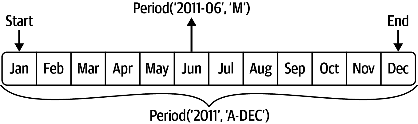
When you are converting from high to low frequency, pandas determines the subperiod, depending on where the superperiod “belongs.” For example, in A-JUN frequency, the month Aug-2011 is actually part of the 2012 period:
In [168]: p = pd.Period("Aug-2011", "M")

In [169]: p.asfreq("A-JUN")
Out[169]: Period('2012', 'A-JUN')
Whole PeriodIndex objects or time series can be similarly converted with the same semantics:
In [170]: periods = pd.period_range("2006", "2009", freq="A-DEC")

In [171]: ts = pd.Series(np.random.standard_normal(len(periods)), index=periods)

In [172]: ts
Out[172]:
2006    1.607578
2007    0.200381
2008   -0.834068
2009   -0.302988
Freq: A-DEC, dtype: float64

In [173]: ts.asfreq("M", how="start")
Out[173]:
2006-01    1.607578
2007-01    0.200381
2008-01   -0.834068
2009-01   -0.302988
Freq: M, dtype: float64
Here, the annual periods are replaced with monthly periods corresponding to the first month falling within each annual period. If we instead wanted the last business day of each year, we can use the "B" frequency and indicate that we want the end of the period:
In [174]: ts.asfreq("B", how="end")
Out[174]:
2006-12-29    1.607578
2007-12-31    0.200381
2008-12-31   -0.834068
2009-12-31   -0.302988
Freq: B, dtype: float64
Quarterly Period Frequencies
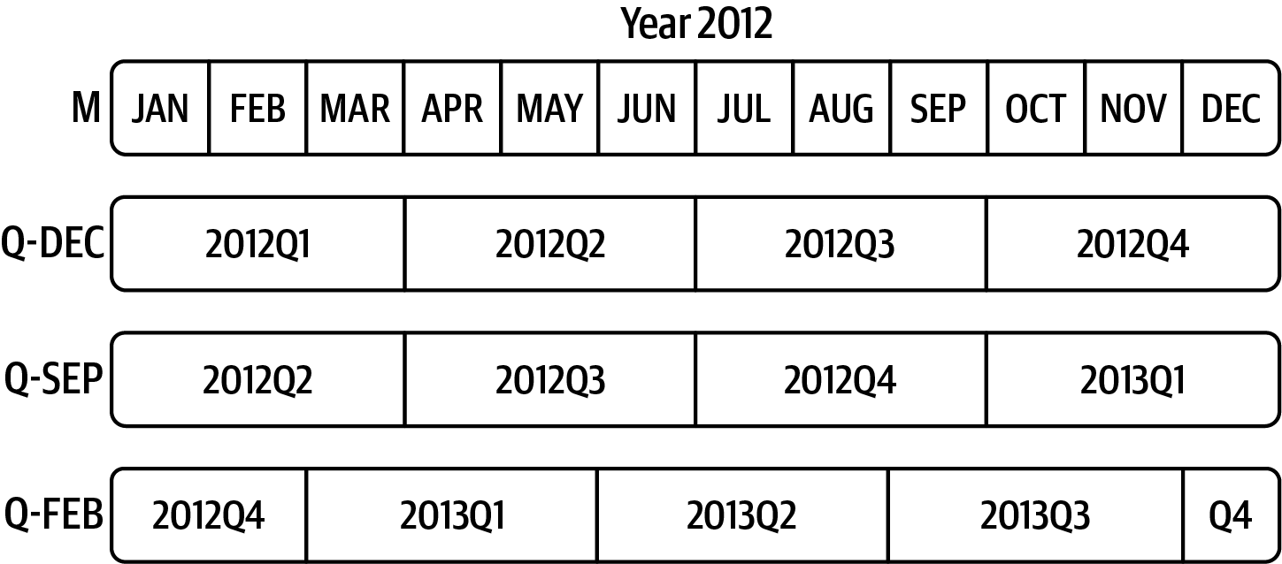
Quarterly data is standard in accounting, finance, and other fields. Much quarterly data is reported relative to a fiscal year end, typically the last calendar or business day of one of the 12 months of the year. Thus, the period 2012Q4 has a different meaning depending on fiscal year end. pandas supports all 12 possible quarterly frequencies as Q-JAN through Q-DEC:
In [175]: p = pd.Period("2012Q4", freq="Q-JAN")

In [176]: p
Out[176]: Period('2012Q4', 'Q-JAN')
In the case of a fiscal year ending in January, 2012Q4 runs from November 2011 through January 2012, which you can check by converting to daily frequency:
In [177]: p.asfreq("D", how="start")
Out[177]: Period('2011-11-01', 'D')

In [178]: p.asfreq("D", how="end")
Out[178]: Period('2012-01-31', 'D')
See Figure 11.2 for an illustration.
Thus, it’s possible to do convenient period arithmetic; for example, to get the timestamp at 4 P.M. on the second-to-last business day of the quarter, you could do:
In [179]: p4pm = (p.asfreq("B", how="end") - 1).asfreq("T", how="start") + 16 * 6
0

In [180]: p4pm
Out[180]: Period('2012-01-30 16:00', 'T')

In [181]: p4pm.to_timestamp()
Out[181]: Timestamp('2012-01-30 16:00:00')
The to_timestamp method returns the Timestamp at the start of the period by default.
You can generate quarterly ranges using pandas.period_range. The arithmetic is identical, too:
In [182]: periods = pd.period_range("2011Q3", "2012Q4", freq="Q-JAN")

In [183]: ts = pd.Series(np.arange(len(periods)), index=periods)

In [184]: ts
Out[184]:
2011Q3    0
2011Q4    1
2012Q1    2
2012Q2    3
2012Q3    4
2012Q4    5
Freq: Q-JAN, dtype: int64

In [185]: new_periods = (periods.asfreq("B", "end") - 1).asfreq("H", "start") + 1
6

In [186]: ts.index = new_periods.to_timestamp()

In [187]: ts
Out[187]:
2010-10-28 16:00:00    0
2011-01-28 16:00:00    1
2011-04-28 16:00:00    2
2011-07-28 16:00:00    3
2011-10-28 16:00:00    4
2012-01-30 16:00:00    5
dtype: int64
Converting Timestamps to Periods (and Back)
Series and DataFrame objects indexed by timestamps can be converted to periods with the to_period method:
In [188]: dates = pd.date_range("2000-01-01", periods=3, freq="M")

In [189]: ts = pd.Series(np.random.standard_normal(3), index=dates)

In [190]: ts
Out[190]:
2000-01-31    1.663261
2000-02-29   -0.996206
2000-03-31    1.521760
Freq: M, dtype: float64

In [191]: pts = ts.to_period()

In [192]: pts
Out[192]:
2000-01    1.663261
2000-02   -0.996206
2000-03    1.521760
Freq: M, dtype: float64
Since periods refer to nonoverlapping time spans, a timestamp can only belong to a single period for a given frequency. While the frequency of the new PeriodIndex is inferred from the timestamps by default, you can specify any supported frequency (most of those listed in Table 11.4 are supported). There is also no problem with having duplicate periods in the result:
In [193]: dates = pd.date_range("2000-01-29", periods=6)

In [194]: ts2 = pd.Series(np.random.standard_normal(6), index=dates)

In [195]: ts2
Out[195]:
2000-01-29    0.244175
2000-01-30    0.423331
2000-01-31   -0.654040
2000-02-01    2.089154
2000-02-02   -0.060220
2000-02-03   -0.167933
Freq: D, dtype: float64

In [196]: ts2.to_period("M")
Out[196]:
2000-01    0.244175
2000-01    0.423331
2000-01   -0.654040
2000-02    2.089154
2000-02   -0.060220
2000-02   -0.167933
Freq: M, dtype: float64
To convert back to timestamps, use the to_timestamp method, which returns a DatetimeIndex:
In [197]: pts = ts2.to_period()

In [198]: pts
Out[198]:
2000-01-29    0.244175
2000-01-30    0.423331
2000-01-31   -0.654040
2000-02-01    2.089154
2000-02-02   -0.060220
2000-02-03   -0.167933
Freq: D, dtype: float64

In [199]: pts.to_timestamp(how="end")
Out[199]:
2000-01-29 23:59:59.999999999    0.244175
2000-01-30 23:59:59.999999999    0.423331
2000-01-31 23:59:59.999999999   -0.654040
2000-02-01 23:59:59.999999999    2.089154
2000-02-02 23:59:59.999999999   -0.060220
2000-02-03 23:59:59.999999999   -0.167933
Freq: D, dtype: float64
Creating a PeriodIndex from Arrays
Fixed frequency datasets are sometimes stored with time span information spread across multiple columns. For example, in this macroeconomic dataset, the year and quarter are in different columns:
In [200]: data = pd.read_csv("examples/macrodata.csv")

In [201]: data.head(5)
Out[201]:
   year  quarter   realgdp  realcons  realinv  realgovt  realdpi    cpi
0  1959        1  2710.349    1707.4  286.898   470.045   1886.9  28.98  \
1  1959        2  2778.801    1733.7  310.859   481.301   1919.7  29.15
2  1959        3  2775.488    1751.8  289.226   491.260   1916.4  29.35
3  1959        4  2785.204    1753.7  299.356   484.052   1931.3  29.37
4  1960        1  2847.699    1770.5  331.722   462.199   1955.5  29.54
      m1  tbilrate  unemp      pop  infl  realint
0  139.7      2.82    5.8  177.146  0.00     0.00
1  141.7      3.08    5.1  177.830  2.34     0.74
2  140.5      3.82    5.3  178.657  2.74     1.09
3  140.0      4.33    5.6  179.386  0.27     4.06
4  139.6      3.50    5.2  180.007  2.31     1.19

In [202]: data["year"]
Out[202]:
0      1959
1      1959
2      1959
3      1959
4      1960
       ...
198    2008
199    2008
200    2009
201    2009
202    2009
Name: year, Length: 203, dtype: int64

In [203]: data["quarter"]
Out[203]:
0      1
1      2
2      3
3      4
4      1
      ..
198    3
199    4
200    1
201    2
202    3
Name: quarter, Length: 203, dtype: int64
By passing these arrays to PeriodIndex with a frequency, you can combine them to form an index for the DataFrame:
In [204]: index = pd.PeriodIndex(year=data["year"], quarter=data["quarter"],
   .....:                        freq="Q-DEC")

In [205]: index
Out[205]:
PeriodIndex(['1959Q1', '1959Q2', '1959Q3', '1959Q4', '1960Q1', '1960Q2',
             '1960Q3', '1960Q4', '1961Q1', '1961Q2',
             ...
             '2007Q2', '2007Q3', '2007Q4', '2008Q1', '2008Q2', '2008Q3',
             '2008Q4', '2009Q1', '2009Q2', '2009Q3'],
            dtype='period[Q-DEC]', length=203)

In [206]: data.index = index

In [207]: data["infl"]
Out[207]:
1959Q1    0.00
1959Q2    2.34
1959Q3    2.74
1959Q4    0.27
1960Q1    2.31
          ...
2008Q3   -3.16
2008Q4   -8.79
2009Q1    0.94
2009Q2    3.37
2009Q3    3.56
Freq: Q-DEC, Name: infl, Length: 203, dtype: float64
11.6 Resampling and Frequency Conversion
Resampling refers to the process of converting a time series from one frequency to another. Aggregating higher frequency data to lower frequency is called downsampling, while converting lower frequency to higher frequency is called upsampling. Not all resampling falls into either of these categories; for example, converting W-WED (weekly on Wednesday) to W-FRI is neither upsampling nor downsampling.
pandas objects are equipped with a resample method, which is the workhorse function for all frequency conversion. resample has a similar API to groupby; you call resample to group the data, then call an aggregation function:
In [208]: dates = pd.date_range("2000-01-01", periods=100)

In [209]: ts = pd.Series(np.random.standard_normal(len(dates)), index=dates)

In [210]: ts
Out[210]:
2000-01-01    0.631634
2000-01-02   -1.594313
2000-01-03   -1.519937
2000-01-04    1.108752
2000-01-05    1.255853
                ...
2000-04-05   -0.423776
2000-04-06    0.789740
2000-04-07    0.937568
2000-04-08   -2.253294
2000-04-09   -1.772919
Freq: D, Length: 100, dtype: float64

In [211]: ts.resample("M").mean()
Out[211]:
2000-01-31   -0.165893
2000-02-29    0.078606
2000-03-31    0.223811
2000-04-30   -0.063643
Freq: M, dtype: float64

In [212]: ts.resample("M", kind="period").mean()
Out[212]:
2000-01   -0.165893
2000-02    0.078606
2000-03    0.223811
2000-04   -0.063643
Freq: M, dtype: float64
resample is a flexible method that can be used to process large time series. The examples in the following sections illustrate its semantics and use. Table 11.5 summarizes some of its options.
| Argument | Description |
|---|---|
rule |
String, DateOffset, or timedelta indicating desired resampled frequency (for example, ’M', ’5min', or Second(15)) |
axis |
Axis to resample on; default axis=0 |
fill_method |
How to interpolate when upsampling, as in "ffill" or "bfill"; by default does no interpolation |
closed |
In downsampling, which end of each interval is closed (inclusive), "right" or "left" |
label |
In downsampling, how to label the aggregated result, with the "right" or "left" bin edge (e.g., the 9:30 to 9:35 five-minute interval could be labeled 9:30 or 9:35) |
limit |
When forward or backward filling, the maximum number of periods to fill |
kind |
Aggregate to periods ("period") or timestamps ("timestamp"); defaults to the type of index the time series has |
convention |
When resampling periods, the convention ("start" or "end") for converting the low-frequency period to high frequency; defaults to "start" |
origin |
The "base" timestamp from which to determine the resampling bin edges; can also be one of "epoch", "start", "start_day", "end", or "end_day"; see the resample docstring for full details |
offset |
An offset timedelta added to the origin; defaults to None |
Downsampling
Downsampling is aggregating data to a regular, lower frequency. The data you’re aggregating doesn’t need to be fixed frequently; the desired frequency defines bin edges that are used to slice the time series into pieces to aggregate. For example, to convert to monthly, "M" or "BM", you need to chop up the data into one-month intervals. Each interval is said to be half-open; a data point can belong only to one interval, and the union of the intervals must make up the whole time frame. There are a couple things to think about when using resample to downsample data:
Which side of each interval is closed
How to label each aggregated bin, either with the start of the interval or the end
To illustrate, let’s look at some one-minute frequency data:
In [213]: dates = pd.date_range("2000-01-01", periods=12, freq="T")

In [214]: ts = pd.Series(np.arange(len(dates)), index=dates)

In [215]: ts
Out[215]:
2000-01-01 00:00:00     0
2000-01-01 00:01:00     1
2000-01-01 00:02:00     2
2000-01-01 00:03:00     3
2000-01-01 00:04:00     4
2000-01-01 00:05:00     5
2000-01-01 00:06:00     6
2000-01-01 00:07:00     7
2000-01-01 00:08:00     8
2000-01-01 00:09:00     9
2000-01-01 00:10:00    10
2000-01-01 00:11:00    11
Freq: T, dtype: int64
Suppose you wanted to aggregate this data into five-minute chunks or bars by taking the sum of each group:
In [216]: ts.resample("5min").sum()
Out[216]:
2000-01-01 00:00:00 10
2000-01-01 00:05:00 35
2000-01-01 00:10:00 21
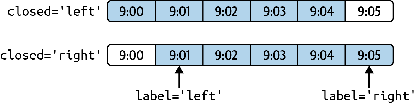
Freq: 5T, dtype: int64The frequency you pass defines bin edges in five-minute increments. For this frequency, by default the left bin edge is inclusive, so the 00:00 value is included in the 00:00 to 00:05 interval, and the 00:05 value is excluded from that interval.1
In [217]: ts.resample("5min", closed="right").sum()
Out[217]:
1999-12-31 23:55:00     0
2000-01-01 00:00:00    15
2000-01-01 00:05:00    40
2000-01-01 00:10:00    11
Freq: 5T, dtype: int64
The resulting time series is labeled by the timestamps from the left side of each bin. By passing label="right" you can label them with the right bin edge:
In [218]: ts.resample("5min", closed="right", label="right").sum()
Out[218]:
2000-01-01 00:00:00     0
2000-01-01 00:05:00    15
2000-01-01 00:10:00    40
2000-01-01 00:15:00    11
Freq: 5T, dtype: int64
See Figure 11.3 for an illustration of minute frequency data being resampled to five-minute frequency.
Lastly, you might want to shift the result index by some amount, say subtracting one second from the right edge to make it more clear which interval the timestamp refers to. To do this, add an offset to the resulting index:
In [219]: from pandas.tseries.frequencies import to_offset

In [220]: result = ts.resample("5min", closed="right", label="right").sum()

In [221]: result.index = result.index + to_offset("-1s")

In [222]: result
Out[222]:
1999-12-31 23:59:59     0
2000-01-01 00:04:59    15
2000-01-01 00:09:59    40
2000-01-01 00:14:59    11
Freq: 5T, dtype: int64
Open-high-low-close (OHLC) resampling
In finance, a popular way to aggregate a time series is to compute four values for each bucket: the first (open), last (close), maximum (high), and minimal (low) values. By using the ohlc aggregate function, you will obtain a DataFrame having columns containing these four aggregates, which are efficiently computed in a single function call:
In [223]: ts = pd.Series(np.random.permutation(np.arange(len(dates))), index=date
s)

In [224]: ts.resample("5min").ohlc()
Out[224]:
                     open  high  low  close
2000-01-01 00:00:00     8     8    1      5
2000-01-01 00:05:00     6    11    2      2
2000-01-01 00:10:00     0     7    0      7
Upsampling and Interpolation
Upsampling is converting from a lower frequency to a higher frequency, where no aggregation is needed. Let’s consider a DataFrame with some weekly data:
In [225]: frame = pd.DataFrame(np.random.standard_normal((2, 4)),
   .....:                      index=pd.date_range("2000-01-01", periods=2,
   .....:                                          freq="W-WED"),
   .....:                      columns=["Colorado", "Texas", "New York", "Ohio"])

In [226]: frame
Out[226]:
            Colorado     Texas  New York      Ohio
2000-01-05 -0.896431  0.927238  0.482284 -0.867130
2000-01-12  0.493841 -0.155434  1.397286  1.507055
When you are using an aggregation function with this data, there is only one value per group, and missing values result in the gaps. We use the asfreq method to convert to the higher frequency without any aggregation:
In [227]: df_daily = frame.resample("D").asfreq()

In [228]: df_daily
Out[228]:
            Colorado     Texas  New York      Ohio
2000-01-05 -0.896431  0.927238  0.482284 -0.867130
2000-01-06       NaN       NaN       NaN       NaN
2000-01-07       NaN       NaN       NaN       NaN
2000-01-08       NaN       NaN       NaN       NaN
2000-01-09       NaN       NaN       NaN       NaN
2000-01-10       NaN       NaN       NaN       NaN
2000-01-11       NaN       NaN       NaN       NaN
2000-01-12  0.493841 -0.155434  1.397286  1.507055
Suppose you wanted to fill forward each weekly value on the non-Wednesdays. The same filling or interpolation methods available in the fillna and reindex methods are available for resampling:
In [229]: frame.resample("D").ffill()
Out[229]:
            Colorado     Texas  New York      Ohio
2000-01-05 -0.896431  0.927238  0.482284 -0.867130
2000-01-06 -0.896431  0.927238  0.482284 -0.867130
2000-01-07 -0.896431  0.927238  0.482284 -0.867130
2000-01-08 -0.896431  0.927238  0.482284 -0.867130
2000-01-09 -0.896431  0.927238  0.482284 -0.867130
2000-01-10 -0.896431  0.927238  0.482284 -0.867130
2000-01-11 -0.896431  0.927238  0.482284 -0.867130
2000-01-12  0.493841 -0.155434  1.397286  1.507055
You can similarly choose to only fill a certain number of periods forward to limit how far to continue using an observed value:
In [230]: frame.resample("D").ffill(limit=2)
Out[230]:
            Colorado     Texas  New York      Ohio
2000-01-05 -0.896431  0.927238  0.482284 -0.867130
2000-01-06 -0.896431  0.927238  0.482284 -0.867130
2000-01-07 -0.896431  0.927238  0.482284 -0.867130
2000-01-08       NaN       NaN       NaN       NaN
2000-01-09       NaN       NaN       NaN       NaN
2000-01-10       NaN       NaN       NaN       NaN
2000-01-11       NaN       NaN       NaN       NaN
2000-01-12  0.493841 -0.155434  1.397286  1.507055
Notably, the new date index need not coincide with the old one at all:
In [231]: frame.resample("W-THU").ffill()
Out[231]:
            Colorado     Texas  New York      Ohio
2000-01-06 -0.896431  0.927238  0.482284 -0.867130
2000-01-13  0.493841 -0.155434  1.397286  1.507055
Resampling with Periods
Resampling data indexed by periods is similar to timestamps:
In [232]: frame = pd.DataFrame(np.random.standard_normal((24, 4)),
   .....:                      index=pd.period_range("1-2000", "12-2001",
   .....:                                            freq="M"),
   .....:                      columns=["Colorado", "Texas", "New York", "Ohio"])

In [233]: frame.head()
Out[233]:
         Colorado     Texas  New York      Ohio
2000-01 -1.179442  0.443171  1.395676 -0.529658
2000-02  0.787358  0.248845  0.743239  1.267746
2000-03  1.302395 -0.272154 -0.051532 -0.467740
2000-04 -1.040816  0.426419  0.312945 -1.115689
2000-05  1.234297 -1.893094 -1.661605 -0.005477

In [234]: annual_frame = frame.resample("A-DEC").mean()

In [235]: annual_frame
Out[235]:
      Colorado     Texas  New York      Ohio
2000  0.487329  0.104466  0.020495 -0.273945
2001  0.203125  0.162429  0.056146 -0.103794
Upsampling is more nuanced, as before resampling you must make a decision about which end of the time span in the new frequency to place the values. The convention argument defaults to "start" but can also be "end":
# Q-DEC: Quarterly, year ending in December
In [236]: annual_frame.resample("Q-DEC").ffill()
Out[236]:
        Colorado     Texas  New York      Ohio
2000Q1  0.487329  0.104466  0.020495 -0.273945
2000Q2  0.487329  0.104466  0.020495 -0.273945
2000Q3  0.487329  0.104466  0.020495 -0.273945
2000Q4  0.487329  0.104466  0.020495 -0.273945
2001Q1  0.203125  0.162429  0.056146 -0.103794
2001Q2  0.203125  0.162429  0.056146 -0.103794
2001Q3  0.203125  0.162429  0.056146 -0.103794
2001Q4  0.203125  0.162429  0.056146 -0.103794

In [237]: annual_frame.resample("Q-DEC", convention="end").asfreq()
Out[237]:
        Colorado     Texas  New York      Ohio
2000Q4  0.487329  0.104466  0.020495 -0.273945
2001Q1       NaN       NaN       NaN       NaN
2001Q2       NaN       NaN       NaN       NaN
2001Q3       NaN       NaN       NaN       NaN
2001Q4  0.203125  0.162429  0.056146 -0.103794
Since periods refer to time spans, the rules about upsampling and downsampling are more rigid:
In downsampling, the target frequency must be a subperiod of the source frequency.
In upsampling, the target frequency must be a superperiod of the source frequency.
If these rules are not satisfied, an exception will be raised. This mainly affects the quarterly, annual, and weekly frequencies; for example, the time spans defined by Q-MAR only line up with A-MAR, A-JUN, A-SEP, and A-DEC:
In [238]: annual_frame.resample("Q-MAR").ffill()
Out[238]:
        Colorado     Texas  New York      Ohio
2000Q4  0.487329  0.104466  0.020495 -0.273945
2001Q1  0.487329  0.104466  0.020495 -0.273945
2001Q2  0.487329  0.104466  0.020495 -0.273945
2001Q3  0.487329  0.104466  0.020495 -0.273945
2001Q4  0.203125  0.162429  0.056146 -0.103794
2002Q1  0.203125  0.162429  0.056146 -0.103794
2002Q2  0.203125  0.162429  0.056146 -0.103794
2002Q3  0.203125  0.162429  0.056146 -0.103794
Grouped Time Resampling
For time series data, the resample method is semantically a group operation based on a time intervalization. Here's a small example table:
In [239]: N = 15

In [240]: times = pd.date_range("2017-05-20 00:00", freq="1min", periods=N)

In [241]: df = pd.DataFrame({"time": times,
   .....:                    "value": np.arange(N)})

In [242]: df
Out[242]:
                  time  value
0  2017-05-20 00:00:00      0
1  2017-05-20 00:01:00      1
2  2017-05-20 00:02:00      2
3  2017-05-20 00:03:00      3
4  2017-05-20 00:04:00      4
5  2017-05-20 00:05:00      5
6  2017-05-20 00:06:00      6
7  2017-05-20 00:07:00      7
8  2017-05-20 00:08:00      8
9  2017-05-20 00:09:00      9
10 2017-05-20 00:10:00     10
11 2017-05-20 00:11:00     11
12 2017-05-20 00:12:00     12
13 2017-05-20 00:13:00     13
14 2017-05-20 00:14:00     14
Here, we can index by "time" and then resample:
In [243]: df.set_index("time").resample("5min").count()
Out[243]:
                     value
time
2017-05-20 00:00:00      5
2017-05-20 00:05:00      5
2017-05-20 00:10:00      5
Suppose that a DataFrame contains multiple time series, marked by an additional group key column:
In [244]: df2 = pd.DataFrame({"time": times.repeat(3),
   .....:                     "key": np.tile(["a", "b", "c"], N),
   .....:                     "value": np.arange(N * 3.)})

In [245]: df2.head(7)
Out[245]:
                 time key  value
0 2017-05-20 00:00:00   a    0.0
1 2017-05-20 00:00:00   b    1.0
2 2017-05-20 00:00:00   c    2.0
3 2017-05-20 00:01:00   a    3.0
4 2017-05-20 00:01:00   b    4.0
5 2017-05-20 00:01:00   c    5.0
6 2017-05-20 00:02:00   a    6.0
To do the same resampling for each value of "key", we introduce the pandas.Grouper object:
In [246]: time_key = pd.Grouper(freq="5min")We can then set the time index, group by "key" and time_key, and aggregate:
In [247]: resampled = (df2.set_index("time")
   .....:              .groupby(["key", time_key])
   .....:              .sum())

In [248]: resampled
Out[248]:
                         value
key time
a   2017-05-20 00:00:00   30.0
    2017-05-20 00:05:00  105.0
    2017-05-20 00:10:00  180.0
b   2017-05-20 00:00:00   35.0
    2017-05-20 00:05:00  110.0
    2017-05-20 00:10:00  185.0
c   2017-05-20 00:00:00   40.0
    2017-05-20 00:05:00  115.0
    2017-05-20 00:10:00  190.0

In [249]: resampled.reset_index()
Out[249]:
  key                time  value
0   a 2017-05-20 00:00:00   30.0
1   a 2017-05-20 00:05:00  105.0
2   a 2017-05-20 00:10:00  180.0
3   b 2017-05-20 00:00:00   35.0
4   b 2017-05-20 00:05:00  110.0
5   b 2017-05-20 00:10:00  185.0
6   c 2017-05-20 00:00:00   40.0
7   c 2017-05-20 00:05:00  115.0
8   c 2017-05-20 00:10:00  190.0
One constraint with using pandas.Grouper is that the time must be the index of the Series or DataFrame.
11.7 Moving Window Functions
An important class of array transformations used for time series operations are statistics and other functions evaluated over a sliding window or with exponentially decaying weights. This can be useful for smoothing noisy or gappy data. I call these moving window functions, even though they include functions without a fixed-length window like exponentially weighted moving average. Like other statistical functions, these also automatically exclude missing data.
Before digging in, we can load up some time series data and resample it to business day frequency:
In [250]: close_px_all = pd.read_csv("examples/stock_px.csv",
   .....:                            parse_dates=True, index_col=0)

In [251]: close_px = close_px_all[["AAPL", "MSFT", "XOM"]]

In [252]: close_px = close_px.resample("B").ffill()
I now introduce the rolling operator, which behaves similarly to resample and groupby. It can be called on a Series or DataFrame along with a window (expressed as a number of periods; see Apple price with 250-day moving average for the plot created):
In [253]: close_px["AAPL"].plot()
Out[253]: <Axes: >

In [254]: close_px["AAPL"].rolling(250).mean().plot()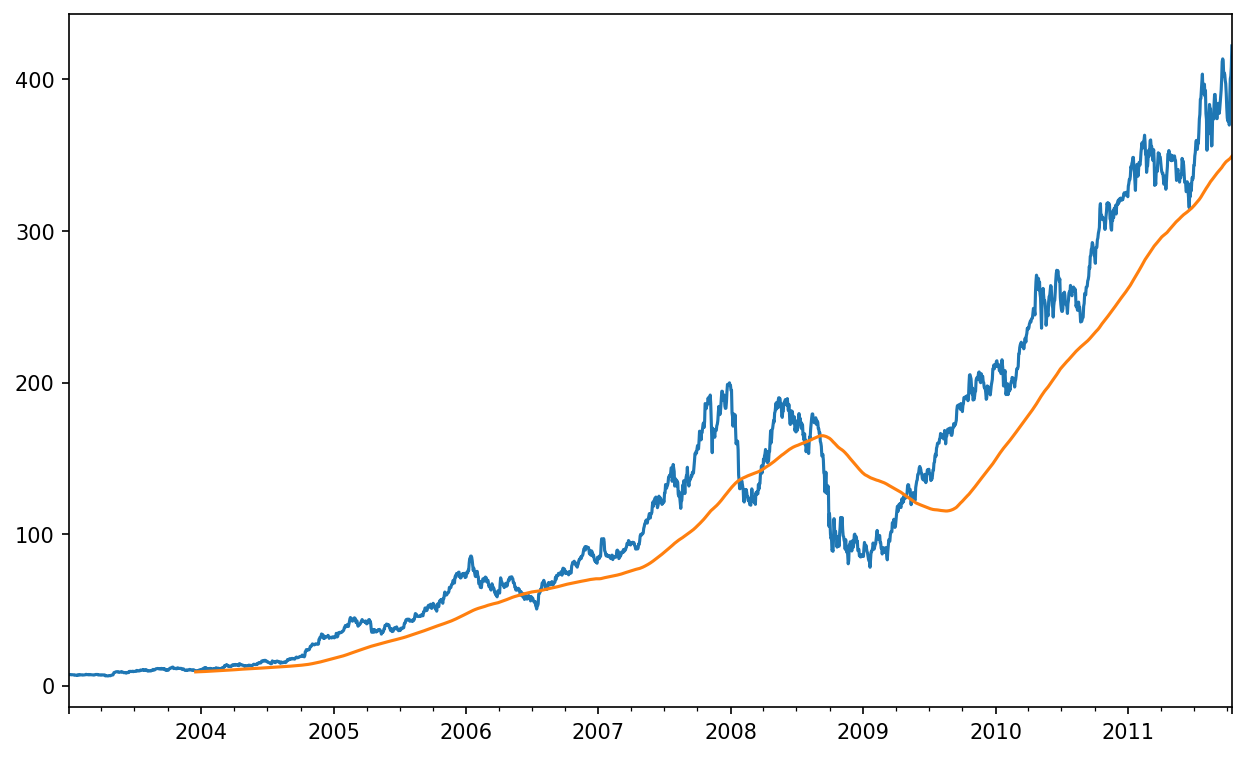
The expression rolling(250) is similar in behavior to groupby, but instead of grouping, it creates an object that enables grouping over a 250-day sliding window. So here we have the 250-day moving window average of Apple's stock price.
By default, rolling functions require all of the values in the window to be non-NA. This behavior can be changed to account for missing data and, in particular, the fact that you will have fewer than window periods of data at the beginning of the time series (see Apple 250-day daily return standard deviation):
In [255]: plt.figure()
Out[255]: <Figure size 1000x600 with 0 Axes>

In [256]: std250 = close_px["AAPL"].pct_change().rolling(250, min_periods=10).std
()

In [257]: std250[5:12]
Out[257]:
2003-01-09         NaN
2003-01-10         NaN
2003-01-13         NaN
2003-01-14         NaN
2003-01-15         NaN
2003-01-16    0.009628
2003-01-17    0.013818
Freq: B, Name: AAPL, dtype: float64

In [258]: std250.plot()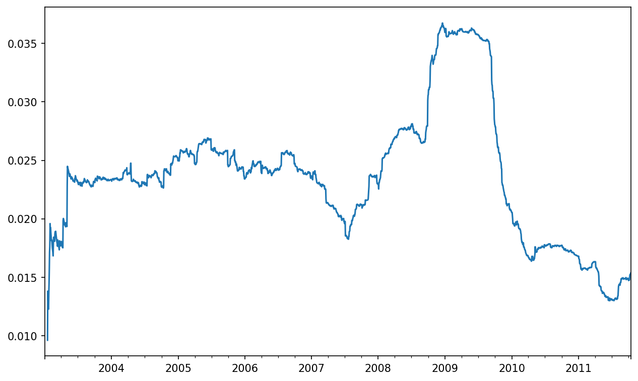
To compute an expanding window mean, use the expanding operator instead of rolling. The expanding mean starts the time window from the same point as the rolling window and increases the size of the window until it encompasses the whole series. An expanding window mean on the std250 time series looks like this:
In [259]: expanding_mean = std250.expanding().mean()Calling a moving window function on a DataFrame applies the transformation to each column (see Stock prices 60-day moving average (log y-axis)):
In [261]: plt.style.use('grayscale')

In [262]: close_px.rolling(60).mean().plot(logy=True)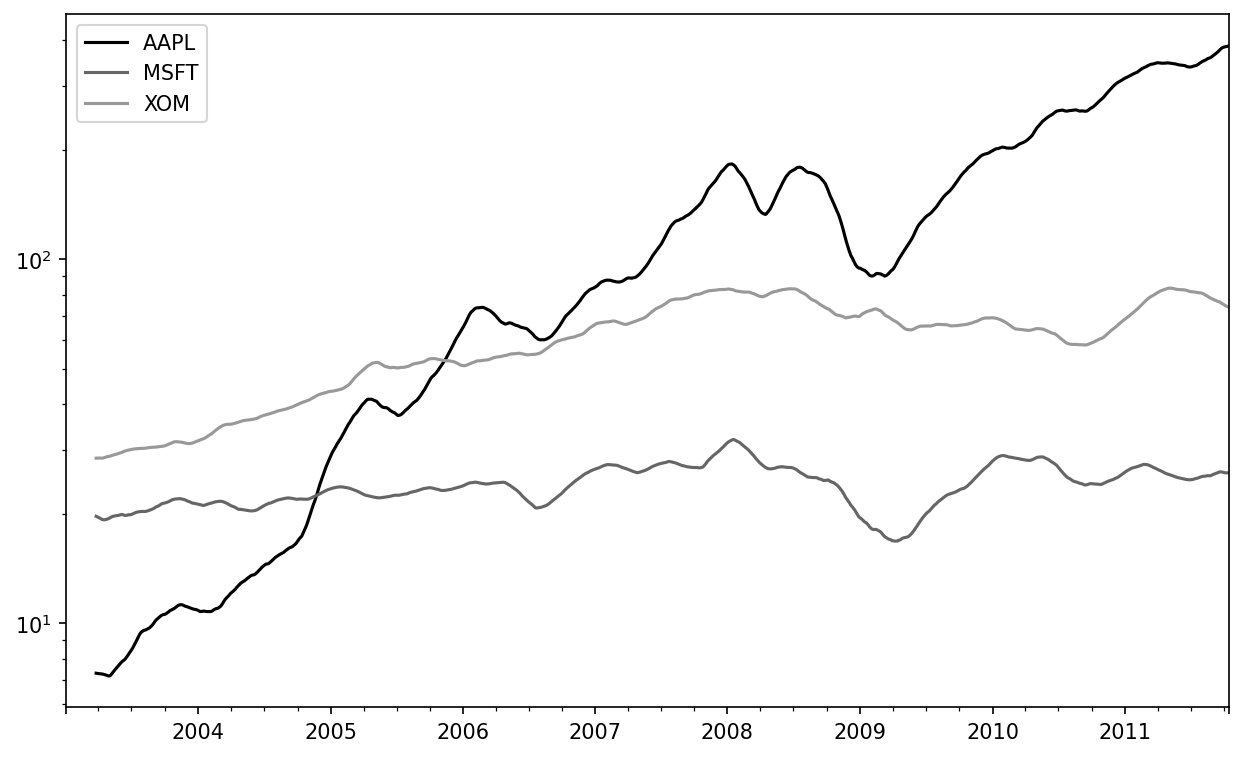
The rolling function also accepts a string indicating a fixed-size time offset rolling() in moving window functions rather than a set number of periods. Using this notation can be useful for irregular time series. These are the same strings that you can pass to resample. For example, we could compute a 20-day rolling mean like so:
In [263]: close_px.rolling("20D").mean()
Out[263]:
                  AAPL       MSFT        XOM
2003-01-02    7.400000  21.110000  29.220000
2003-01-03    7.425000  21.125000  29.230000
2003-01-06    7.433333  21.256667  29.473333
2003-01-07    7.432500  21.425000  29.342500
2003-01-08    7.402000  21.402000  29.240000
...                ...        ...        ...
2011-10-10  389.351429  25.602143  72.527857
2011-10-11  388.505000  25.674286  72.835000
2011-10-12  388.531429  25.810000  73.400714
2011-10-13  388.826429  25.961429  73.905000
2011-10-14  391.038000  26.048667  74.185333
[2292 rows x 3 columns]
Exponentially Weighted Functions
An alternative to using a fixed window size with equally weighted observations is to specify a constant decay factor to give more weight to more recent observations. There are a couple of ways to specify the decay factor. A popular one is using a span, which makes the result comparable to a simple moving window function with window size equal to the span.
Since an exponentially weighted statistic places more weight on more recent observations, it “adapts” faster to changes compared with the equal-weighted version.
pandas has the ewm operator (which stands for exponentially weighted moving) to go along with rolling and expanding. Here’s an example comparing a 30-day moving average of Apple’s stock price with an exponentially weighted (EW) moving average with span=60 (see Simple moving average versus exponentially weighted):
In [265]: aapl_px = close_px["AAPL"]["2006":"2007"]

In [266]: ma30 = aapl_px.rolling(30, min_periods=20).mean()

In [267]: ewma30 = aapl_px.ewm(span=30).mean()

In [268]: aapl_px.plot(style="k-", label="Price")
Out[268]: <Axes: >

In [269]: ma30.plot(style="k--", label="Simple Moving Avg")
Out[269]: <Axes: >

In [270]: ewma30.plot(style="k-", label="EW MA")
Out[270]: <Axes: >

In [271]: plt.legend()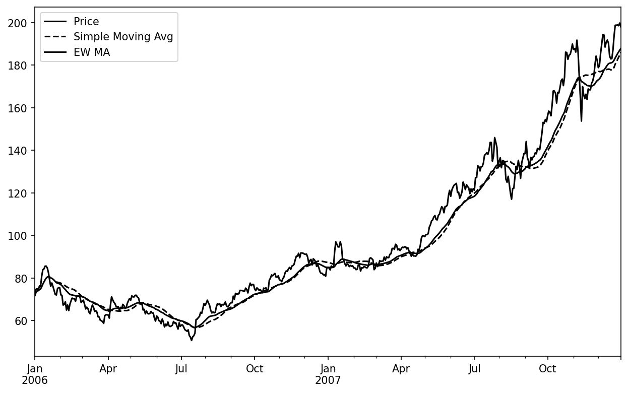
Binary Moving Window Functions
Some statistical operators, like correlation and covariance, need to operate on two time series. As an example, financial analysts are often interested in a stock’s correlation to a benchmark index like the S&P 500. To have a look at this, we first compute the percent change for all of our time series of interest:
In [273]: spx_px = close_px_all["SPX"]

In [274]: spx_rets = spx_px.pct_change()

In [275]: returns = close_px.pct_change()
After we call rolling, the corr aggregation function can then compute the rolling correlation with spx_rets (see Six-month AAPL return correlation to S&P 500 for the resulting plot):
In [276]: corr = returns["AAPL"].rolling(125, min_periods=100).corr(spx_rets)

In [277]: corr.plot()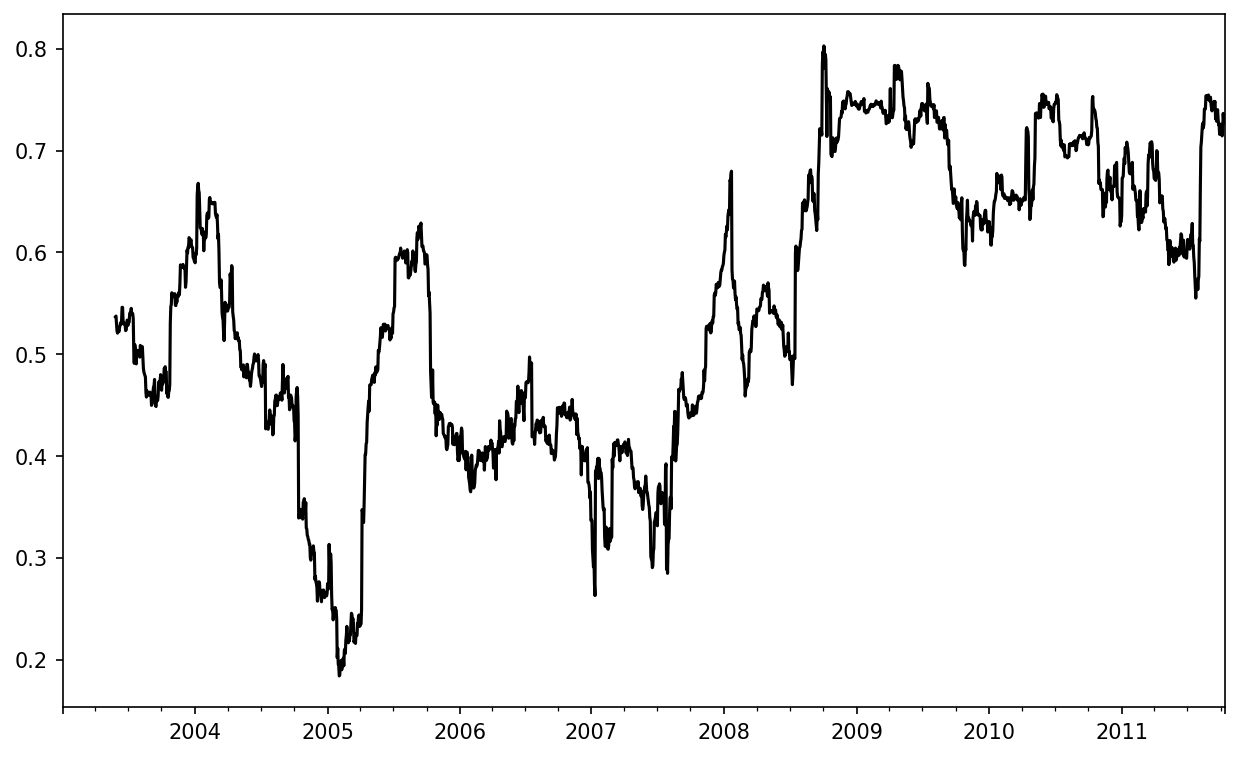
Suppose you wanted to compute the rolling correlation of the S&P 500 index with many stocks at once. You could write a loop computing this for each stock like we did for Apple above, but if each stock is a column in a single DataFrame, we can compute all of the rolling correlations in one shot by calling rolling on the DataFrame and passing the spx_rets Series.
See Six-month return correlations to S&P 500 for the plot of the result:
In [279]: corr = returns.rolling(125, min_periods=100).corr(spx_rets)

In [280]: corr.plot()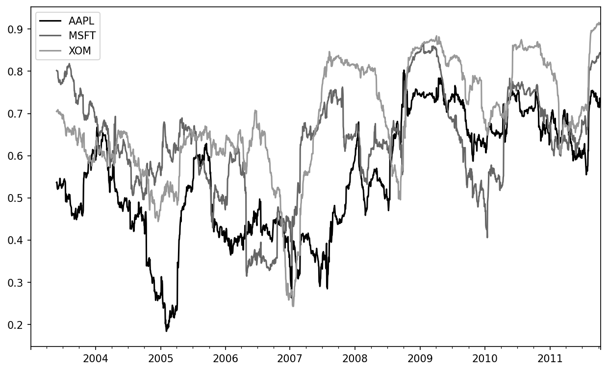
User-Defined Moving Window Functions
The apply method on rolling and related methods provides a way to apply an array function of your own creation over a moving window. The only requirement is that the function produce a single value (a reduction) from each piece of the array. For example, while we can compute sample quantiles using rolling(...).quantile(q), we might be interested in the percentile rank of a particular value over the sample. The scipy.stats.percentileofscore function does just this (see Percentile rank of 2% AAPL return over one-year window for the resulting plot):
In [282]: from scipy.stats import percentileofscore

In [283]: def score_at_2percent(x):
   .....:     return percentileofscore(x, 0.02)

In [284]: result = returns["AAPL"].rolling(250).apply(score_at_2percent)

In [285]: result.plot()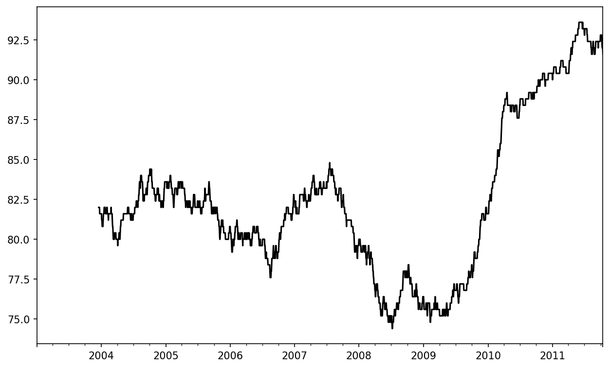
If you don't have SciPy installed already, you can install it with conda or pip:
conda install scipy11.8 Conclusion
Time series data calls for different types of analysis and data transformation tools than the other types of data we have explored in previous chapters.
In the following chapter, we will show how to start using modeling libraries like statsmodels and scikit-learn.
The choice of the default values for
closedandlabelmight seem a bit odd to some users. The default isclosed="left"for all but a specific set ("M","A","Q","BM","BQ", and"W") for which the default isclosed="right". The defaults were chosen to make the results more intuitive, but it is worth knowing that the default is not always one or the other.↩︎